What is the Naive Bayes Algorithm?

It is an algorithm that learns the probability of every object, its features, and which groups they belong to. It is also known as a probabilistic classifier. The Naive Bayes Algorithm comes under supervised learning and is mainly used to solve classification problems.

For example, you cannot identify a bird based on its features and color as there are many birds with similar attributes. But, you make a probabilistic prediction about the same, and that is where the Naive Bayes Algorithm comes in.

Probability, Bayes Theory, and Conditional Probability

Probability is the base for the Naive Bayes algorithm. This algorithm is built based on the probability results that it can offer for unsolvable problems with the help of prediction. You can learn more about probability, Bayes theory, and conditional probability below:

Probability

Probability helps to predict an event's occurrence out of all the potential outcomes. The mathematical equation for probability is as follows:

Probability of an event = Number of Favorable Events/ Total number of outcomes

0 < = probability of an event < = 1. The favorable outcome denotes the event that results from the probability. Probability is always between 0 and 1, where 0 means no probability of it happening, and 1 means the success rate of that event is likely.

For better understanding, you can also consider a case where you predict a fruit based on its color and texture. Here are some possible assumptions that you can make. You can either choose the correct fruit that you have in mind or get confused with similar fruits and make mistakes. Either way, the probability of choosing the right fruit is 50%.

Bayes Theory

Bayes Theory works on coming to a hypothesis (H) from a given set of evidence (E). It relates to two things: the probability of the hypothesis before the evidence P(H) and the probability after the evidence P(H|E). The Bayes Theory is explained by the following equation:

P(H|E) = (P(E|H} * P(H))/P(E)

In the above equation,

• P(H|E) denotes how event H happens when event E takes place.
• P(E|H) represents how often event E happens when event H takes place first.
• P(H) represents the probability of event X happening on its own.
• P(E) represents the probability of event Y happening on its own.

The Bayes Rule is a method for determining P(H|E) from P(E|H). In short, it provides you with a way of calculating the probability of a hypothesis with the provided evidence.

Conditional Probability

Conditional probability is a subset of probability. It reduces the probability of becoming dependent on a single event. You can compute the conditional probability for two or more occurrences.

When you take events X and Y, the conditional probability of event Y is defined as the probability that the event occurs when event X is already over. It is written as P(Y|X). The mathematical formula for this is as follows:

P(Y|A) = P(X and Y) /P(X)

Bayesian Probability

Bayesian Probability allows to calculate the conditional probabilities. It enables to use of partial knowledge for calculating the probability of the occurrence of a specific event. This algorithm is used for developing models for prediction and classification problems like Naive Bayes.

The Bayesian Rule is used in probability theory for computing - conditional probabilities. What is important is that you cannot discover just how the evidence will impact the probability of an event occurring, but you can find the exact probability.

Bayes Theory from a machine learning standpoint

There are training data to train your model and make it functional. You then need to validate the data for evaluating the model and making new predictions. Finally, you need to call the input attributes “evidence” and label them “outputs” in the training data.

Using conditional probability denoted by P(E|O), you can calculate the probability of the evidence from the given outputs. Your ultimate goal is to compute P(O|E) - the probability of output based on the current attributes.

When the problem has two outputs, you can calculate the probability of every outcome and say which one wins. Whereas if you have various input attributes, then the Naive Bayesian Algorithm will be needed.

How Naive Bayes Classifier works?

You can now try to build a classification model that uses Sklearn to see how the Naive Bayes Classifier works. Sklearn is also known as Scikit-Learn. It is an open-source machine-learning library that is written in Python.

For instance, you are using the social_media_ads dataset. With this problem, you can predict if a user has purchased a product by clicking on the ad, depending on her age and other attributes. You can understand the working of the Naive Bayes Classifier by following the below steps:

Step 1 - Import basic libraries

You can use the below command for importing the basic libraries required.

# Importing basic libraries
import numpy as np
import matplotlib.pyplot as plt
import pandas as pd

Step 2 - Importing the dataset

Using the below code, import the dataset, which is required.

# Importing the dataset
dataset = pd.read_csv(‘Social_Media_Ads.csv’)
X = dataset.iloc[:, [3, 4]]
y = dataset.iloc[:, 5]
print(“Prediction evidence:\n”, X.head())
print(“\nFinal Target:\n”, y.head())

Step 3 - Data preprocessing

The below command will help you with the data preprocessing.

# Conversion of variables into arrays
X = X.values
y = y.values
Dataset splitting into training and test datasets(70:30)
from sklearn.selection_of_model import splitting_of_train_test_dataset
X_train, X_test, y_train, y_test = splitting_of_train_test_dataset(X, y, test_size = 0.30)
Feature Scaling
from sklearn.preprocessing import StandardScaler
sc = StandardScaler()
X_train = sc.transform_fit(X_train)
X_test = sc.transform(X_test)

In this step, you have to split the dataset into a training dataset (70%) and a testing dataset (30%). Next, you have to do some basic feature scaling with the help of a standard scaler. It will transform the dataset in a way where the mean value will be 0, and the standard deviation will be 1.

Step 4 - Training the model

You should then write the following command for training the model.

# Fitting of Naive Bayes Algorithm to the Training Dataset

from sklearn.naive_bayes_algorithm import GaussianNB
classifier = GaussianNB()
classifier.fit(X_train, y_train)

Step 5 - Testing and evaluation of the model

The code for testing and evaluating the model is as below:

# Prediction of the test dataset outcomes
y_pred = classifier.predict(X_test)

Constructing the confusion matrix
import seaborn as sns
from sklearn.metrics import confusion_matrix
cm = confusion_matrix(y_test, y_pred)
sns.heatmap(cm, annot=True)

A confusion matrix helps to understand the quality of the model. It describes the production of a classification model on a set of test data for which you know the true values. Every row in a confusion matrix portrays an actual class, and every column portrays the predicted class.

Step 6 - Visualizing the model

Finally, the below code will help in visualizing the model.

# Visualizing the test dataset results

from matplotlib.colors import ColormapListed
X_datsetset, y_datasetset = X_test, y_test
X1, X2 = np.meshgrid(np.arrange(start = X_dataset[:,0].min()-1, stop = X_dataset[:. 0].max() + 1, step =
np.arrange(start = X_dataset[:, 1[.min() -1, stop = X_dataset[:, 1].max() +1, step = 0.02))
plt.contourf(X1, X2, Classifier.predict(np.array([X1.ravel(), X2.ravel()].T).rescape(X1.shape),
alpha = 0.3, cmap = ColormapListed((‘yellow’, ‘blue’)))
plt.xlim(X1.min(), X1.max())
plt.ylim(X2.min(), X2.max())
for u, v in enumerate(np.unique(y_set)):
plt.scatter(X_dataset[y_dataset == v, 0], X_dataset[y_dataset== v, 1],
c = ColormapListed((‘yellow’,’blue’))(i), label = v)
plt.xlabel(‘Current_age’)
plt.ylabel(‘Gross_salary’)
plt.legend()
plt.show()

Code Idea: Towardsdatascience.com

However, in some cases, these steps might not be absolutely necessary. But the above-mentioned example provides a clear idea and information about how data points can be classified.

Types of the Naive Bayes Model

There are four types of the Naive Bayes Model, which are explained below:

Gaussian Naive Bayes

It is a straightforward algorithm used when the attributes are continuous. The attributes present in the data should follow the rule of Gaussian distribution or normal distribution. It remarkably quickens the search, and under lenient conditions, the error will be two times greater than Optimal Naive Bayes.

Optimal Naive Bayes

Optimal Naive Bayes selects the class that has the greatest posterior probability of happenings. As per the name, it is optimal. But it will go through all the possibilities, which is very slow and time-consuming.

Bernoulli Naive Bayes

Bernoulli Naive Bayes is an algorithm that is useful for data that has binary or boolean attributes. The attributes will have a value of yes or no, useful or not, granted or rejected, etc.

Multinominal Naive Bayes

Multinominal Naive Bayes is used on documentation classification issues. The features needed for this type are the frequency of the words converted from the document.

Advantages of a Naive Bayes Classifier

Here are some advantages of the Naive Bayes Classifier:

• It doesn’t require larger amounts of training data.
• It is straightforward to implement.
• Convergence is quicker than other models, which are discriminative.
• It is highly scalable with several data points and predictors.
• It can handle both continuous and categorical data.
• It is not sensitive to irrelevant data and doesn’t follow the assumptions it holds.
• It is used in real-time predictions.

Disadvantages of a Naive Bayes Classifier

The disadvantage of the Naive Bayes Classifier are as below:

• The Naive Bayes Algorithm has trouble with the ‘zero-frequency problem’. It happens when you assign zero probability for categorical variables in the training dataset that is not available. When you use a smooth method for overcoming this problem, you can make it work the best.
• It will assume that all the attributes are independent, which rarely happens in real life. It will limit the application of this algorithm in real-world situations.
• It will estimate things wrong sometimes, so you shouldn’t take its probability outputs seriously.

Applications that use Naive Bayes

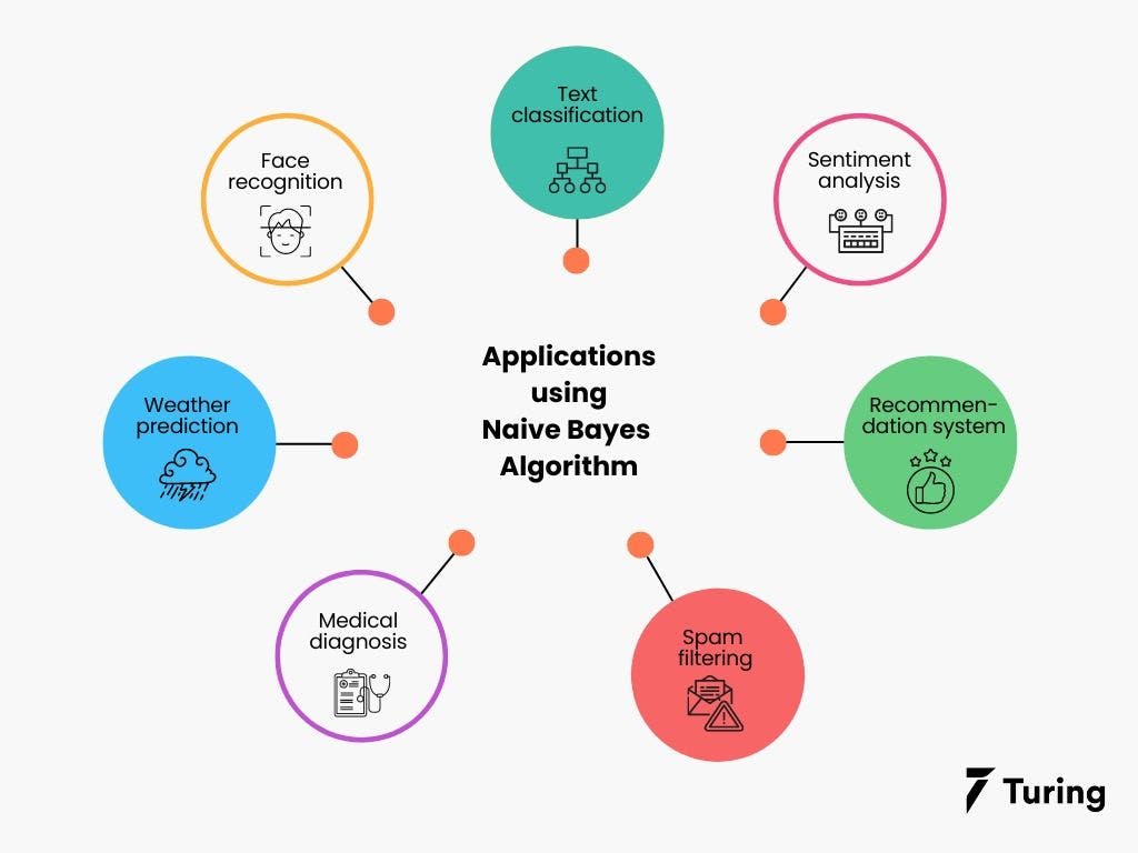
The Naive Bayes Algorithm is used for various real-world problems like those below:

• Text classification: The Naive Bayes Algorithm is used as a probabilistic learning technique for text classification. It is one of the best-known algorithms used for document classification of one or many classes.
• Sentiment analysis: The Naive Bayes Algorithm is used to analyze sentiments or feelings, whether positive, neutral, or negative.
• Recommendation system: The Naive Bayes Algorithm is a collection of collaborative filtering issued for building hybrid recommendation systems that assist you in predicting whether a user will receive any resource.
• Spam filtering: It is also similar to the text classification process. It is popular for helping you determine if the mail you receive is spam.
• Medical diagnosis: This algorithm is used in medical diagnosis and helps you to predict the patient’s risk level for certain diseases.
• Weather prediction: You can use this algorithm to predict whether the weather will be good.
• Face recognition: This helps you identify faces.

Wrapping Up

Though the Naive Bayes Algorithm has a lot of limitations, it is still the most chosen algorithm for solving classification problems because of its simplicity. It works well on spam filtering and the classification of documents. It has the highest rate of success when compared to other algorithms because of its speed and efficiency.