Scikit-Learn Cheatsheet: Methods For Classification and Regression

Machine learning (ML) predictions are based on regression and classifications - the two central pillars of ML tasks - and scikit-learn is the simplest, most efficient, and most widely used library for implementing any ML task. In this article, we will provide a scikit-learn cheatsheet to help you out in every situation!

Resolving everyday problems using ML techniques is rapidly increasing. For example, Gmail uses ML to solve daily issues like sorting mails into spam, promotions, and primary emails. Even in the medical field, researchers are trying to predict the spread of disease among populations with various factors. But how does it work? Through regression and classifications.

What is regression?

Regression is a machine learning method where we train a model with historical data available to make predictions for the unknown future. Common examples of regression tasks include stock market price prediction, estimation of regional sales for various products in a factory, demand prediction for a particular item based on past sales records, and so on.

What is classification?

Classification is where we train a model to classify data into well-defined categories, based on previous data labels. It includes applications like detecting the presence or absence of disease from x-ray data, classifying animal images into different categories, sentiment classification on tweets, movie reviews, and much more.

A brief overview of scikit-learn

Scikit-learn is an open-source Python package. It is a library that provides a set of selected tools for ML and statistical modeling. It includes regression, classification, dimensionality reduction, and clustering. It is properly documented and easy to install and use in a few simple steps.

Scikit-learn for regression

The scikit-learn library provides sample datasets that you can embed and use to familiarize yourself with the package and ML techniques. Here, we will be using the diabetes dataset to perform the regression. It has 10 feature variables about the age, gender, and other clinical data of patients. The target variable is a numerical measure of the diabetes extent in patients. The objective here is to predict the target measures providing the remaining values of the features.

This is how it is done:

Step 1: The first step is to import the libraries and modules. Import the datasets module of sklearn to use the inbuilt data available as shown below:

import sklearn
import pandas as pd
from sklearn import datasets

Step 2: Next, load the diabetes data and set the column names. You can then create a Pandas data frame for the features of the dataset by naming it “diabetes.data”. After that, you can store the target values separately as shown. The code snippet you will get in the output image will be as shown below:

diabetes = datasets.load_diabetes()
columns = "age sex bmi map tc ldl hdl tch ltg glu".split()
x = pd.DataFrame(diabetes.data, columns=columns) 
y = diabetes.target
x.head()

Source: Author’s Kaggle notebook

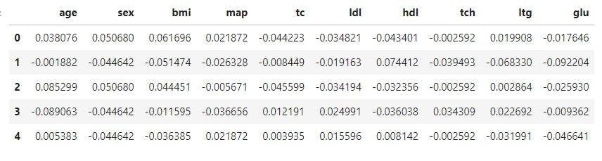
Source: Author’s Kaggle notebook

Here, x has the independent variables and y has the dependent variable. In any modeling, it is a common practice to set aside some amount of data for testing purposes. Sklearn provides an elegant function “train_test_split()” that will randomly split your data into training and testing sets. You can adjust the size of the testing set using the “test_size” parameter.

from sklearn.model_selection import train_test_split
X_train, X_test, y_train, y_test = train_test_split(x, y, test_size=0.2)
print(X_train.shape, y_train.shape)
print(X_test.shape, y_test.shape)

> (353, 10) (353,)
> (89, 10) (89,)

Now that training and testing sets are ready, let's quickly move to the list of models that can be used.

- Linear regression

Linear regression is the most common method for supervised learning. We fit a regression line with the data points available. It is easy to interpret, cost-efficient, and is used as a baseline in any business case.

Import the model class from the linear_model module of sklearn. Initialize and fit it with the training data as shown below:

from sklearn.linear_model import LinearRegression
model = LinearRegression()
model.fit(X_train, y_train)

You can use the trained model to make predictions of unseen data. You can also evaluate it using the inbuilt score function.

predictions = model.predict(X_test)
model.score(X_test, y_test)

- Ridge regression

Ridge regression is an improved version of linear regression. It removes some issues of the OLS (ordinary least squares) methodology. It also imposes a penalty for ranging coefficient values with the alpha parameter. This coefficient plays a vital role in the calculation of the residual sum of squares for ridge regression, making the model robust.

from sklearn import linear_model
model = linear_model.Ridge(alpha=.5)
model.fit(X_train, y_train)

- Polynomial regression

Modern data is often complex with non-linear patterns that cannot be modeled by simple linear models. Polynomial regressions are models where we fit a higher degree curve to the data. It makes the model more flexible and scalable. To implement this in scikit-learn, you have to use the pipeline component. You can define the polynomial degree required in the pipeline.

Follow the below code snippet:

from sklearn.preprocessing import PolynomialFeatures
from sklearn.linear_model import LinearRegression
from sklearn.pipeline import Pipeline
model = Pipeline([('poly', PolynomialFeatures(degree=3)),
        ('linear', LinearRegression(fit_intercept=False))])
model.fit(X_train, y_train)

- Support vector regression (SVR)

SVMs (support vector machines) were initially developed to classify problems, but they have been extended to apply to regression too. These models can be used when you have a higher dimension of features. They also provide different kernel options as per requirements.

The snippet below shows how to import and train an SVR in sklearn:

from sklearn import svm
model = svm.SVR()
model.fit(X_train, y_train)
predictions = model.predict(X_test)

- Decision tree regression

Decision tree regression is a tree-based model where the data is split into subgroups based on homogeneity. You can import this model from the tree module of sklearn.

In order to avoid overfitting, make use of the “max_depth” parameter. It decides the maximum depth of the decision tree. If the value is set too high, the model might fit on noises and perform poorly upon a test dataset.

from sklearn.tree import DecisionTreeRegressor
model = DecisionTreeRegressor(max_depth=12)
model.fit(X_train, y_train)

- Random forest regression

Decision tree models are usually upscaled a level higher by combining multiple models. These are ensemble learning methods. They can be broadly classified into boosting and bagging algorithms.

The base models are weak learners, and by combining multiple weak learners, we get the final, strong learner model. The ‘ensemble’ module has all these functions in sklearn. “N_estimators” is an important parameter that decides the number of decision trees that require training.

from sklearn.ensemble import RandomForestRegressor
model=RandomForestRegressor(n_estimators=10, max_features=2, max_leaf_nodes=5,random_state=42)
model.fit(X_train, y_train)

Scikit learn for classification

Just like for regression, the scikit-learn library provides inbuilt datasets and models for classification tasks. In an example below, we will be using the Iris dataset of sklearn.

The aim is to classify the species of a flower where the features like petal length and width are provided. There are 3 classes of species: sesota, versicolor, and virginica. So, it is a multiclass classification that we are considering here. You can split them into training and testing data sets as usual.

import pandas as pd
from sklearn.datasets import load_iris
iris=load_iris()
x = pd.DataFrame(iris.data) 
y = iris.target 
from sklearn.model_selection import train_test_split
X_train, X_test, y_train, y_test = train_test_split(x, y, test_size=0.2)

Let’s now dive into the various models that sklearn provides.

- Logistic regression

This is a linear model, developed from linear regression to address classification issues. It uses the default regularization technique in the algorithm. When we apply this to multiclass classification problems, it uses the One vs Rest strategy. Here, separate binary classifiers are trained for each class, converting them into a binary classification at the base level.

from sklearn.linear_model import LogisticRegression
clf = LogisticRegression(random_state=13)
clf.fit(X_train, y_train)
predictions = clf.predict(X_test)

- Support vector classifiers

SVM classifiers are popularly used for classification problems with a high dimension of features. They can transform the feature space into a higher dimension using the kernel function. Multiple kernel options are available including linear, RBF (radial base function), polynomial, and so on. We can also finetune the ‘gamma’ parameter, which is the kernel coefficient.

from sklearn.pipeline import make_pipeline
from sklearn.preprocessing import StandardScaler
from sklearn.svm import SVC
clf = make_pipeline(StandardScaler(), SVC(gamma='auto', kernel ='rbf’))
clf.fit(X_train, y_train)

- Naive Bayes classifier

The gaussian Naive Bayes is a popular classification algorithm. It applies Bayes’ theorem of conditional probability to the case. It assumes that the features are independent of each other, while the targets are dependent on them. Have a look at the implementations below:

from sklearn.naive_bayes import GaussianNB
clf = GaussianNB()
clf.fit(X_train, y_train)

- Decision tree classifier

This is a tree-based structure, where a dataset is split based on values of various attributes. Finally, the data points with features of similar values are grouped together. Make sure to finetune the maximum depth and minimum leaf split parameters for better results. It also helps to avoid overfitting.

from sklearn.tree import DecisionTreeClassifier
clf = DecisionTreeClassifier()
clf.fit(X_train, y_train)

- Gradient boosting classifier

Boosting is a method of ensemble learning where multiple decision trees are combined to enhance performance. It is a parallel learning method where multiple trees are trained parallelly and then combined to vote for the final result. We can finetune the hyperparameters like learning rate and number of estimators to achieve optimal training results.

from sklearn.ensemble import GradientBoostingClassifier
clf = GradientBoostingClassifier(n_estimators=100, learning_rate=1.0,max_depth=5, random_state=0)
clf.fit(X_train, y_train)

- KNN classification

KNN (K nearest neighbor) is a classification algorithm that groups data points into clusters. The value of K can be chosen as a parameter “n_neighbors”. The algorithms form K clusters and assign each data point to the nearest cluster.

KNN performs multiple iterations where the distance of the points are the centers of the clusters, which are calculated and reassigned optimally.

from sklearn import neighbors
clf = neighbors.KNeighborsClassifier(n_neighbors=5, weights=distance)
clf.fit(X_train, y_train)

This concludes that the major methods offered in scikit-learn are model regression and classification.

Scikit-learn metrics for evaluation

Modeling is a very significant step in the ML pipeline and so is evaluating it! The good news is that scikit-learn offers multiple functions and metrics to evaluate the predictions for both regression and classification.

Regression metrics

The R squared correlation metric is very popular to start with. Follow the code snippet:

from sklearn.metrics import r2_score
print(r2_score(y_test, y_pred))

The syntax is similar for all the metrics. Below is the list of metrics you can import and test it as required.

from sklearn.metrics import mean_absolute_error
from sklearn.metrics import mean_squared_log_error
from sklearn.metrics import mean_absolute_percentage_error
from sklearn.metrics import median_absolute_error

Classification metrics

For any classification problem, you can generate a classification report with sklearn. This provides information on precision and recalls for each class in the case of a multiclass classification task. It also calculates the F1 score and accuracy of the predictions.

from sklearn.metrics import classification_report
print(classification_report(y_test, y_pred))

A confusion matrix is also a suggested method for classification. It helps you visualize how well the model is performing if there are more false positives or negatives. Sklearn provides a simple way to obtain that too.

from sklearn.metrics import confusion_matrix
print(confusion_matrix( y_test, y_pred))

Machine learning algorithms are truly a vital part of our daily life activities now. Regression and classification being the key of these metrics, we have discussed the models in detail and how the scikit-learn library can help with the practice use cases. There are other metrics that can be explored too like ROC curve, AUC curve, and so on, which will unveil other variations of classification and regression methods.

FAQs

1. What algorithms does Scikit-learn provide?

Scikit-learn provides algorithms like linear regression, logistic regression, decision tree models, random forest regression, gradient boosting regression, gradient boosting classification, K-nearest neighbors, Support Vector Machine, Naive Bayes, neural networks, and a lot more. Broadly, these algorithms could be classified under Supervised (regression, classification) and unsupervised learning (clustering) algorithms.

2. What is the difference between classification and regression in Machine learning?

The difference between classification and regression depends on the properties of the target variable. If the target variable we want to predict is a continuous value it is a regression problem. Whereas, if the target variable is a category that takes values among the N classes, it is a classification problem. Image classification of animals into various categories, text sentiment classification, etc are a few examples.

3. How to split data for training and testing in scikit-learn?

The scikit learn package provides a simple function, “train_test_split()” in its model_selection module. You can provide the size of the test set you want, which will be randomly allocated from the overall training data. This function helps in ensuring that the test set is unbiased, and will serve as a proper evaluation for the algorithm.

4. How to reduce overfitting in scikit learn models?

Overfitting happens when the model you have trained is very complex and has fitted on every training data point. It has memorized the training data, rather than learning the pattern as we desire. To ensure that your model is not overfitting, sklearn provides various hyperparameters you can tune for each model. For example, in decision tree regressions, you can reduce the maximum depth of trees if you find it overfitting. In Support vector machine models, there are regularization parameters like C and gamma to help with this. In neural networks, you can reduce the no of layers, no of neurons in hidden layers and so on.

5. How to evaluate scikit learn models?

There is whole set of metrics available to evaluate your model in the “sklearn.metrics” module. There are metrics available separately for classification and regression problems. Metrics like R squared correlation, Mean Squared Error, Mean Absolute Error, Accuracy are commonly used for regression. Whereas classification problems use metrics like precision, recall, AUC, ROC, IOU (Intersection Over Union), and so on.