A Beginner’s Guide to Complete Mathematical Intuition Behind Linear Regression Algorithm.

How should you decide when to use a linear regression model? How does a system decide the best fit line, the error and how it can be minimized? This article will provide answers to these questions and an understanding of the linear regression approach as a whole.
Let’s dive in.

What is linear regression?

Linear regression is a procedure used in statistics. As the term implies, it can only be used when there is a linear relationship among the variables, ie., when there is a straight-line relationship between two variables.

Image source

It’s used as a model for understanding the association between independent and dependent variables as well as to foresee the connection between two quantitative variables: predictor variables, which are known as independent variables, and dependent variables, which are those being predicted. For example, you want to predict the price of a house based on its Area, Garage Area, Land Contour, Utilities, etc. Here, "price" will be the dependent variable and "Area, Garage Area, Land Contour, Utilities" will be the independent variable.

Real-life examples of regression

Example #1
Businesses frequently use linear regression to comprehend the connection between advertising spending and revenue. For instance, they might apply the linear regression model using advertising spend as an independent variable or predictor variable and revenue as the response variable. The equation would take the following form:

revenue = β0 + β1 (ad. spending)

Example #2
Linear regression may be used in the medical field to understand the relationships between drug dosage and patient blood pressure. Researchers may manage different measurements of a specific medication to patients and see how their circulatory strain reacts/blood pressure responds. They might fit a model using dosage as an independent variable and blood pressure as the dependent variable. The equation would be:

blood pressure = β0 + β1 (dosage)

Example #3
Agriculture scientists frequently use linear regression to see the impact of rainfall and fertilizer on the amount of fruits/vegetables yielded. For instance, scientists might use different amounts of fertilizer and see the effect of rain on different fields and to ascertain how it affects crop yield. They might fit a multiple linear regression using rainfall and fertilizer as the predictor variables and crop yield as the dependent variable or response variable. The regression model would take the following form:

crop yield = β0 + β1 (rainfall) + β2(fertilizer)

Different names of linear regression

Linear regression has been around since 1805. It has been studied from every possible angle and each has a different name such as linear regression, multiple linear regression, polynomial regression, etc. The main aim behind every regression model is to predict a value using some features.

An easy way to know which is which is this: it’s called linear regression when there’s a single independent variable. When there are more than two independent variables, it’s called multiple linear regression.

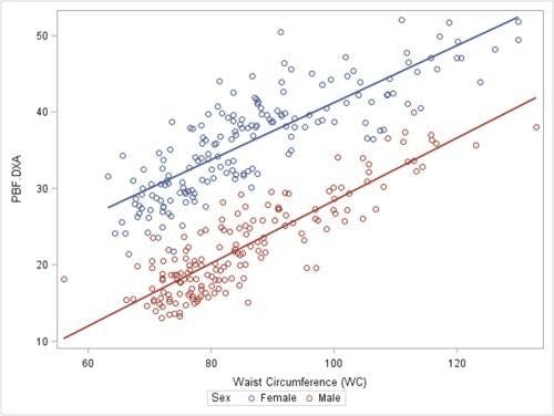
Linear regression is only applied when there is a linear relationship among variables. A simple way to check this relationship is to make a pair plot or scatter plot between the variables. The graph will show if linear regression is applicable or not.

What kind of relationship can linear regression show?

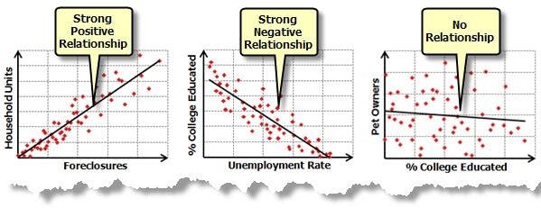
• Positive relationship

When the regression line between the two variables moves in the same direction with an upward slope, the variables are said to be in a positive relationship. This means that if the value of x (independent variable) is increased, there will be an increase in the dependent variable.

• Negative relationship

When the regression line between the two variables moves in the same direction with a downward slope, the variables are said to be in a negative relationship. This shows that if the value of the independent variable (x) is increased, there will be a decrease in the dependent variable (y).

• No relationship

If the best fit line is flat (not sloped), it’s assumed that there is no relationship among the variables. There will be no change in the dependent variable (y) by increasing or decreasing the independent variable (x) value.

You can determine what kind of relationship these variables have by using correlation or covariance.
Covariance shows the direction of the relationship between X and Y but it doesn't say how positive or negative the relationship is. To know this, remember that if the covariance value is negative and if the independent variable (X) increases, the dependent variable (Y) decreases and vice versa.
Correlation is a statistical measure that shows the direction of the relationship as well as the strength of the relationship (how positively or negatively the variables are correlated) . The range of correlation is between -1<correlation< +1. It’s called a perfect correlation if all points fall on the best fit line - which is very unlikely.

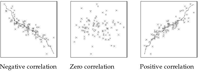
Image source: docs.oracle.com

Least square method

The main idea behind the linear regression model is to fit a line that is the best fit for the data. For this, you use a technique called least square method. In layman's terms, it is the process of fitting the best curve for a set of data points by reducing the distance between the actual value and predicted value (sum of squared residuals). The distance between both values is often known as error or variation or variance.

It’s known that the equation of a straight line is y = a + bx.

Similarly, the equation of the best fit line for linear regression is:

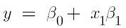
Image source: Author

Meanwhile, since there are more than 2 independent variables in multiple linear regression, the equation becomes:

Image source: Author

where β0 is the Y-intercept of the regression line
β1 is the slope of the regression line
Xi is the explanatory variable.

The next question is, what error is this? Can it be visualized? How can it be found? Fortunately, there’s no need to worry about the mathematics of a linear model as everything is done by the model itself.

Image source: Author

In the graph above, the best fit line will be similar. The only difference will be the number of data points.
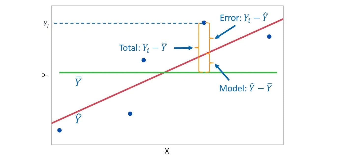
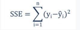
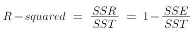
Suppose there's a variable Yi. The distance between Yi and the predicted value is what is called “sum of squared estimate of errors” or SSE. This is the unexplained variance and it must be minimized to get the best accuracy.

Image source: Author

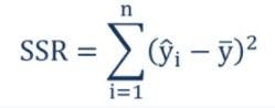
The distance between the predicted value y_hat and the mean of dependent variable is called ”sum of squared residuals” or SSR. This is the explained variance of the model and it should be maximized.
An advantage of this error is that it can be used as the loss function since it is differentiable at all points. The disadvantage is that it is not robust to outliers.

Image source: Author

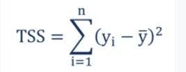
The total variation in the model (SSR+SSE=SST) is called the”sum of squared total”.

Image source: Author

How do you do linear regression?

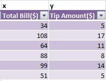
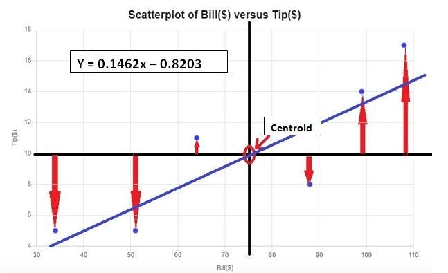
Here’s an example: you want to know to what degree the tip amount can be predicted by the bill studied. The tip is the dependent variable (response variable) and the bill is the independent variable (predictor variable).

Image source: Author

To fit the best fit line, you need to minimize the sum of squared errors, which is the distance between the predicted value and actual value.

Step 1: Check if there is a linear relationship between the variables.

You already know that the equation of a line is y=mx+c or y = x*β1+β0. Make a scatter plot to see a relationship between the variables. Remember that the best fit line will always pass through the centroid, which is the intersection of x_bar and y_bar.

Image source: Author

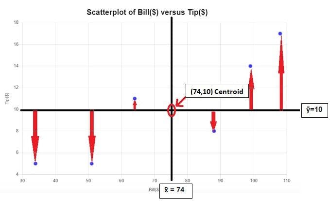
You can see that there is a positive relationship. As the bill amount is increased, there is an increase in the tip amount too. Hence, you can use linear regression to predict the response variable.

Step 2: Check the correlation of the data.

After plotting a scatter plot and knowing what type of relationship it has, calculate the correlation to know the direction’s strength. In this case, the correlation is 0.866, which shows that the relationship is very strong.

Step 3: Calculations.

Now that you know that the relationship is positive and very strong, it’s time to start the calculations.
The equation of best-fit line is: Ŷ = x*β1+β0
where β1 is the coefficient of regression or slope. To predict Ŷ, you need to know this coefficient. It will also tell you the change in dependent variable if you increase the independent variable by 1 unit. The formula for finding this is:

Image source: Author

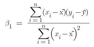
and if the constant term is calculated by β0=ȳ-x̄*β1

Image source: Author

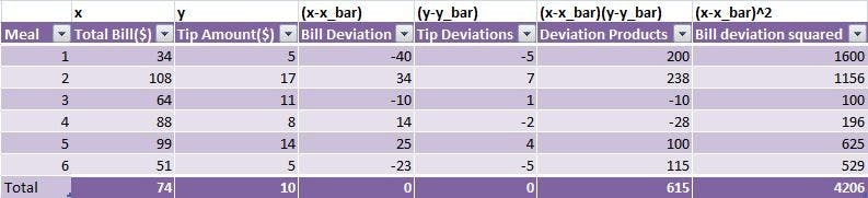
You get x̄ = 74, ȳ = 10 , Σ (x-x̄)(y-ȳ) = 615 , Σ (x-x̄)^2 = 4206.
Putting all the values in β1, you get β1 0.1462. This means that if you increase the bill by 1 unit, the tip amount will increase by 0.1462 units.
Similarly, β0 = -0.8203. The intercept may or may not have any meaning in real life.
Hence, the equation of the best fit line is Ŷ = 0.1462x - 0.8203.

Since there are so many calculations, you can use Python libraries to make the work easier.
The next session will interpret the results of a linear regression on a medical cost dataset. Here is the full EDA and code.

Image source: Author

Interpretation of linear regression result

Image source: Author

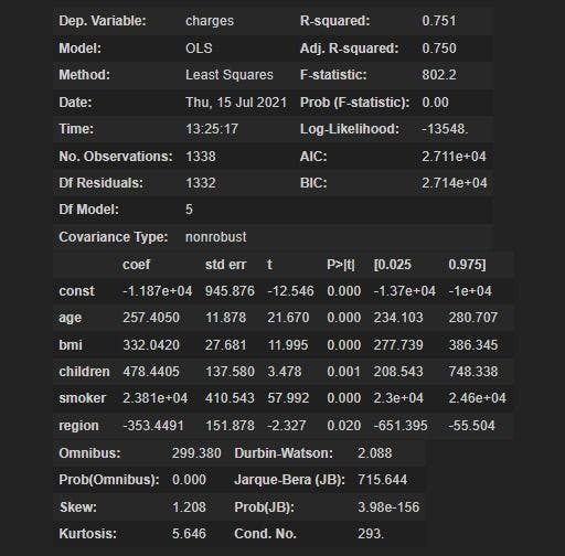
To see the summary of your linear regression model, run the following code:

import statsmodels.api as sm
X = sm.add_constant(x)

model = sm.ols(y,x).fit()

model.summary()

ANOVA

Image source: Author

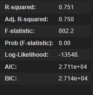
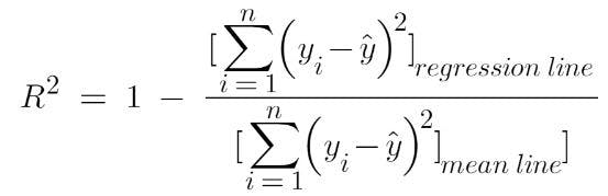
Coefficient of determination (R-squared)

R-squared states the proportion of the variability explained by the model, i.e what percent of the model represents the real-life model. Here’s an example:
You have an independent variable as “CGPA” and a dependent variable as “Package”. You want to apply to xyz college and know the package you will receive after graduating. Since you haven’t mentioned your CGPA or anything to help them give an accurate answer, they will tell you the average package of their previous students. But, suppose you give your CGPA and ask the same question, they will be able to predict the package. In essence, they will fit a linear regression line to their previous data to arrive at an answer.

The R2 score shows the superior results that linear regression can give instead of basing them on the mean of other students.

Image source: Author

Image source: Author

where it is used to know the accuracy of the model.
The range of R square is from 0-1, but can it go below 0? When will this value be 1 and what will that mean?

• Can R square be 0?

Yes, if both the lines have the same error. If the regression line comes upon the mean line, you can say that both have the same error. This means that giving the college your CGPA has no importance because you will get the same result even without that information.

• Can R square be 1?

Yes. For this to happen, you need the ratio of the regression line error and the mean line error to be equal to 0. It can be 0 only when the error of the regression line is 0. This will happen when the regression line perfectly fits all the points, which is rare.

• Can R square value be -1 or any negative value?

Yes, but only when the ratio of the regression line error and the mean line error is greater than 1. And this can happen only when SSR > SST. This means that the linear regression line error is more than the worst-case scenario and this can happen only when the regression line doesn’t touch a single point.

Here, you can see that the R square value is 0.751, which means that the model could explain 75.1% variance in the data or that the fitted values represent the original values with good accuracy. Since it is a tabular dataset, the values are continuous and the target column must have varying values. By looking at this value, you can say that the features provided to the model were able to explain 75.1% of the variability. You can’t say anything about the remaining 25%.

Note that a good model has a high R-squared value. But how high is high?
R square > 80% implies the model is a good fit.
60% < R square < 80% implies the model is an okay fit.
R square < 60% implies the model needs improvement.
If your R-squared value is less, you may need to check your independent variables again and see if there are any outliers.

Adjusted R-squared

Every time you add a new input variable, there will be an increase in the R square. Hence, it’s not wise to use the R square to decide whether to add a new input variable. To address this, a quantity known as "adjusted R-squared", which is a modified version of R-squared, is used. It’s more useful when you add irrelevant variables to the model. If you add variables that do not affect the target variable, the adjusted R-squared value will decrease and R-squared value will increase. Note that it is always lower than the R square.

Usually, the value of R-squared and adjusted R-squared is somewhat the same. But, if you see a large difference, you need to check your independent variables again and see if there is any relationship between the target variable and the independent variable.

Image source: Author

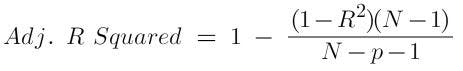
where R square = Coefficient of determination
N = Total sample size
p = number of predictors (independent variables) in the model.

F-statistic: The value of F-statistic here reveals that not every one of the coefficients of the model may be equivalent to 0. If the overall F-test is significant, you can conclude that R-squared does not equal 0 and that the correlation between the model and dependent variable is statistically significant.

The null hypothesis here is (H0): The model with no independent variables fits the data as well as the model.

The alternate hypothesis (H1): The model fits the data better than the intercept-only model.

The p-value helps check whether there is enough evidence to accept the alternate hypothesis. If you are testing at a 95% confidence interval then, if:

p-value < level of significance (in this case 5%), you can reject H0.
p-value > level of significance, you cannot reject H0.

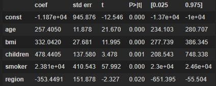
Variables

Image source: Author

Let's interpret this and see what can be derived. Keep in mind that you need to have rudimentary knowledge of statistics to better understand Machine Learning.

Coefficient: The coefficient of a variable shows that if you increase the independent variable by 1 unit, holding other variables of the model constant (remember, linear regression assumes that there is no multicollinearity in the model, so independent variables have no collinearity between them), then the dependent variable will increase by that much value.

The table shows that the coefficient of age is 257.4050, so if you increase age by 1 year the target variable will increase by 257.4050. If there was a negative coefficient - for example, coefficient of "region" - you would say that increasing the value of the region by 1 unit will see a decrease of -353.4491 in the target variable.

Coefficients can also highlight how significant the variable is for the model. If the coefficient value is close to 0, you can say that there is no relationship between the variable and the target variable.

Standard error: In order to understand standard error, you need to know about standard deviation. Standard deviation tells the variation of the values from the mean or how spread the data is. About 95% of the values lie within 2 standard deviations of the mean.

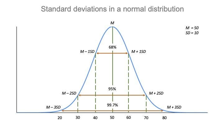
To interpret standard error in layman’s terms, let’s use a population and pick 10 samples. If you find the mean of these samples and plot them on a standard normal graph, the standard deviation of these samples is what is called a standard error. It will show how accurate the mean of any given sample is from the true population.

Image source: Author

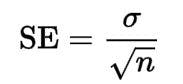
Here in the regression model, the standard error gives the estimated standard deviation of the distribution of coefficients.

Confusing? Here’s a breakdown:

For every 1 unit increase in age, the target variable will go up by 257.4050. If you re-run the model, the standard error will show that there may be some variation in this coefficient. For example, in age, the standard error of 11.878 shows that the coefficient of age may vary by 11.878 if you re-run the model.

Here’s the result again:

Image source: Author

t-stat - t-statistic or t-value is calculated by dividing the coefficient from the standard error.

t-stat = Coefficient/Std.Error
The value of the t-statistic will help determine if the coefficient value is really that number or if it happened by chance. If the value of t-statistic is greater than the tabulated value

Image source: Author

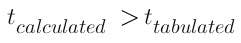
you will reject the null hypothesis since the value falls under the rejection area.
The null hypothesis (H0): each of the coefficients at population level is 0.
The alternate hypothesis (H1): the coefficients are not 0 at population level.
The higher the value of t-statistic in magnitude, the more significant the variable is.

P > |t| - p-value is the probability for the null hypothesis to be true. If you look at the p-value of age, you can see that the probability that the null hypothesis is true is approximately equal to 0. P-value will show that it is very unlikely that there is no relationship between the independent variable and the dependent variable, which means that the coefficients are not 0 at the population level.

Typically, a p-value of 5% or less is a good cut-off point. If the p-value is greater than 0.05 (p-value>0.05), then fail to reject the null hypothesis and say that there is no relationship between the variable and the target variable. If it is less than 0.05 (p-value<0.05), reject the null hypothesis and say that the coefficients are not equal to 0.

The higher the value of t-statistic, the lower will be the p-value and the higher will be the chances that the value of the coefficients are significant and didn't happen by chance.

Congratulations on learning to interpret the linear regression model from scratch! It’s always better to know what’s happening under the hood. It’s important to understand what these terms inform in this model as only then will you be able to proceed and make good predictions.