Softmax: Multiclass Neural Networks

Softmax activation function or normalized exponential function is a generalization of the logistic function that turns a vector of K real values into a vector of K real values that sum to 1. Even if the input values are negative, zero, positive, or greater than one, the softmax function transforms every value between 0 and 1. This is done in order to interpret them as probabilities.

If any of the inputs is negative or small in value, the softmax function turns it into a small probability. Conversely, if the input value is enormous, it turns it into a large probability. The values, however, will always remain between 0 and 1.

What are the variants of softmax function?

The softmax function has a couple of variants: full softmax and candidate sampling.

1. Full softmax

This variant of softmax calculates the probability of every possible class. We will use it the most when dealing with multiclass neural networks in Python. It is quite cheap when used with a small number of classes. However, it becomes expensive as soon as the number of classes increases.

2. Candidate sampling

In this variant of the softmax function, only the calculation of the probability of positive labels takes place. However, it does so only for a random sample of negative labels. The idea behind this variant is that the negative classes can learn from the less frequent negative reinforcement.

Candidate sampling can be done as long as the positive classes get adequate positive reinforcement. Obviously, this needs to be observed empirically to ensure computational efficiency. Overall, however, it adds to the efficiency of the output when there are many classes to be dealt with.

For example, if we are interested in determining whether the input image is an apple or a mango, we don’t have to provide the probabilities for a non-fruit example.

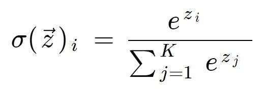
What is the mathematical representation of softmax?

Here’s the mathematical representation of the softmax function:

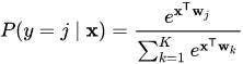
Here’s another mathematical expression for the softmax function which extends the formula for logistic regression into multiple classes given below:

Image source

Image source

The softmax function extends this thought into a multiclass classification world. It assigns decimal probabilities to every class included in a multi-class problem. Since each of them would lie between 0 and 1, the decimal probabilities must add up to 1.

Softmax finds application in several subjects, including multiclass neural networks. We will now dig deeper into this ‌application.

Multiclass neural networks

In a multiclass neural network in Python, we resolve a classification problem with N potential solutions. It utilizes the approach of one versus all and leverages binary classification for each likely outcome.

One v/s many labels

Softmax considers that every example is a member of only one class. However, in cases when an example is a member of multiple classes, we may not be able to use the softmax function on them. We will have to rely on multiple logistic regressions for the same.

For instance, consider that you have a set of examples with exactly one item as a piece of fruit. The softmax function can easily evaluate the likelihood of one item being a mango, an orange, an apple, and so on. But if the examples are images that contain bowls of different kinds of fruits, you will be able to determine the likelihood of that one item you are looking for with the help of multiple logistic regressions.

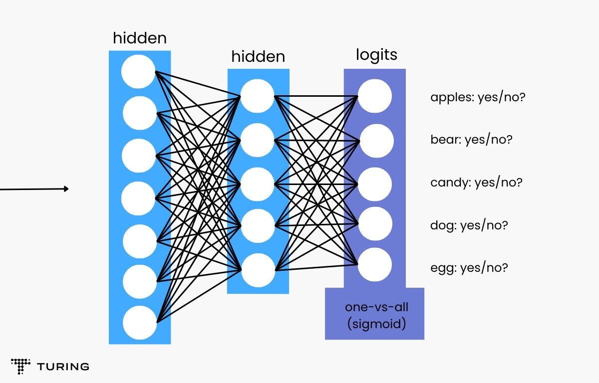
Now, consider that you input a picture of a dog and train the model with five different binary recognizers.

Note: A binary classifier that accepts two inputs comprises a hidden layer of 128 neurons.

Here is the code for a binary classifier that outputs values between 0 and 1, depicting that the input belongs to the positive class:

model = Sequential()
model.add(Dense(128, activation='relu', input_dim=2))
model.add(Dense(1, activation='sigmoid'))
model.compile(optimizer='adam', loss=' binary_crossentropy', metrics=['accuracy'])

Code source

Here’s how the binary classifiers will see the image and offer their responses:

1. Is there an apple in the image? No.
2. Is there a bear in the image? No.
3. Is there candy in the image? No.
4. Is there a dog in the image? Yes.
5. Is there an egg in the image? No.

Here’s a figure that explains this approach in a more efficient one-vs-all model with a deep softmax neural network:

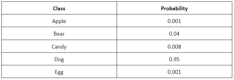
With this, a softmax function would produce the following probabilities that belong to a particular class:

Remember that we implement the softmax function before the output layer through a neural network layer. We need to ensure that the softmax layer has the same number of norms as that in the output layer.

The figure below gives a clearer picture:

Note: Such an approach is only beneficial when the total number of classes is small. When the number of classes increases, we will need a higher sequence of binary classifiers to improve the accuracy of the output.

Understanding the calculation of softmax in a neural network

Let’s explore the calculation with a convolutional softmax neural network that recognizes if an image is of a cat or a dog. Note that the image cannot be both and must be ‌either one of them, making the two classes mutually exclusive.

If we look at the final fully connected layer of this network, we will receive an output like [-7.98, 2.39] that cannot be interpreted as probabilities. However, by adding a layer of softmax function to the network, these numbers can be translated into a probability distribution. This means that the output can be fed to the machine learning algorithms and we can receive guaranteed results between 0 and 1. There is no need to normalize the values.

Note: In miscellaneous cases, such as when there is no cat or dog in the image, the network will be forced to categorize it into one. So, to allow the possibility of output for such a case, we need to re-configure the multiclass neural network to have a third output.

Let us assume class 1 to be for cats and class 2 to be for a dog. If we input a cat image, ideally the network will output [1,0] and for a dog image [0,1].

Remember that the neural network image processing stops at the final fully connected layer. We will receive two outputs which are not probabilities for a cat and a dog. The usual practice is to include a softmax layer at the end of the neural network to get the output in the form of probability.

Initially, when the neural network weights are randomly configured, both the images go through and get converted by the image processing stage to scores [1.2, 0.3]. So when we pass these scores into the softmax function, we get the initial probabilities as [0.71, 0.29].

The mathematical representation below provides a better understanding:

Code source

Code source

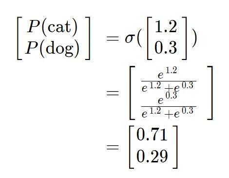
We have discussed that a perfect network would put forward an output of [1,0] in this scenario. In order to bring the output probabilities [0.71, 0.29] closest to [1,0], we adjust the weights of the model accordingly.

To do this, we formulate a loss function of a network that calculates the extent to which the network's output probability varies from the desired values.

We choose the most common loss function, cross-entropy loss, to calculate how much output varies from the desired output.

Code source

Code source

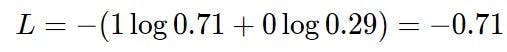
If the value of the loss function is small, the output vector is closer to the correct class and vice versa.

Since the softmax activation function is our continuously differentiable function, we can calculate the derivative of the loss function for every weight or for every image in the training set. It allows us to reduce the loss function and improve the network's accuracy by bringing the network's output closer to the desired value of the network.

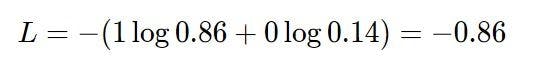
Now, we update the networks after several iterations of training. When we input the same cat into the network, we receive a score vector of [1.9, 0.1] at the end of the fully connected layer. To get these in the format of probabilities, we put them through the softmax function again.

Code source

Code source

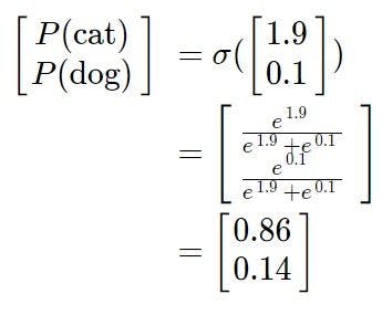
For now, the results received are much closer to the desired output of [1,0]. If we calculate the cross-entropy loss again, we will notice that the loss value is decreased. It is more acceptable and accurate as compared to the last output received.

Code source

Code source

The softmax function has applications in a variety of operations, including facial recognition. Its journey from its source in statistical mechanics as the Boltzmann distribution in the foundational paper Boltzmann (1868) to its present use in machine learning and other subjects is recommendable. It can be used to derive accurate results from any number of classes on the table.