Transfer Learning Using CNN (VGG16)

Transfer learning is one of the handiest tools to use if you’re working on any sort of image classification problem. But what exactly is it? How can you implement it? How accurate is it? This article will go in-depth into transfer learning and show you how to apply it using the Keras library.

Note that a prerequisite to learning transfer learning is to have basic knowledge of convolutional neural networks (CNN) since image classification calls for using this algorithm.

CNNs make use of convolution layers that utilize filters to help recognize the important features in an image. These features, of which there are many, help distinguish a particular image. Whenever you train a CNN on a bunch of images, all these features are learned internally. In addition, when you use a deep CNN, the number of parameters that are being learned - also called weights - can be in the millions. Therefore, when numerous parameters need to be learned, it takes time. And this is where transfer learning helps.

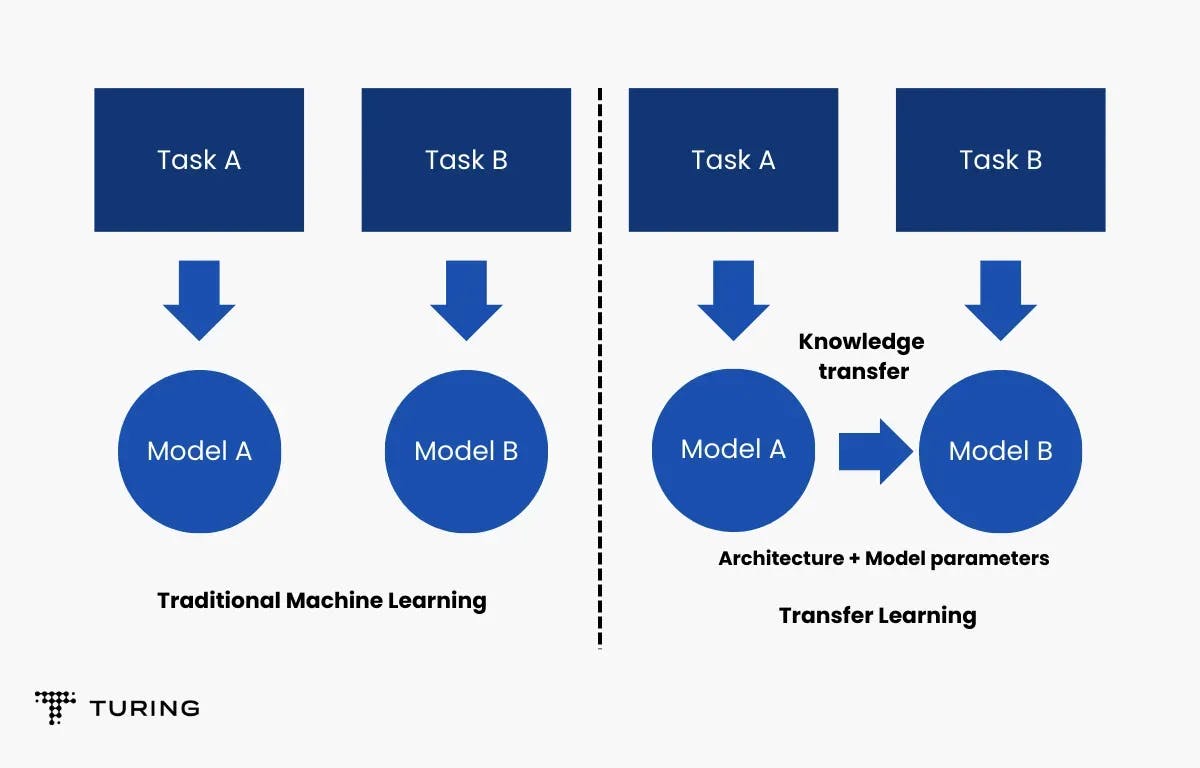
Here’s how.
For example, say there’s a problem called ImageNet classification, a popular image classification challenge where there are millions of images. You need to use these images to predict and classify them into thousands of classes.

Image source

Every year, one model outperforms the other. Once it has been established that a particular model performs the best, all the parameters or all the weights that it has learned are made publicly available. Using Keras application, you can directly use the best model and all the pretrained weights so that you need not run the training process again. This saves a lot of time.

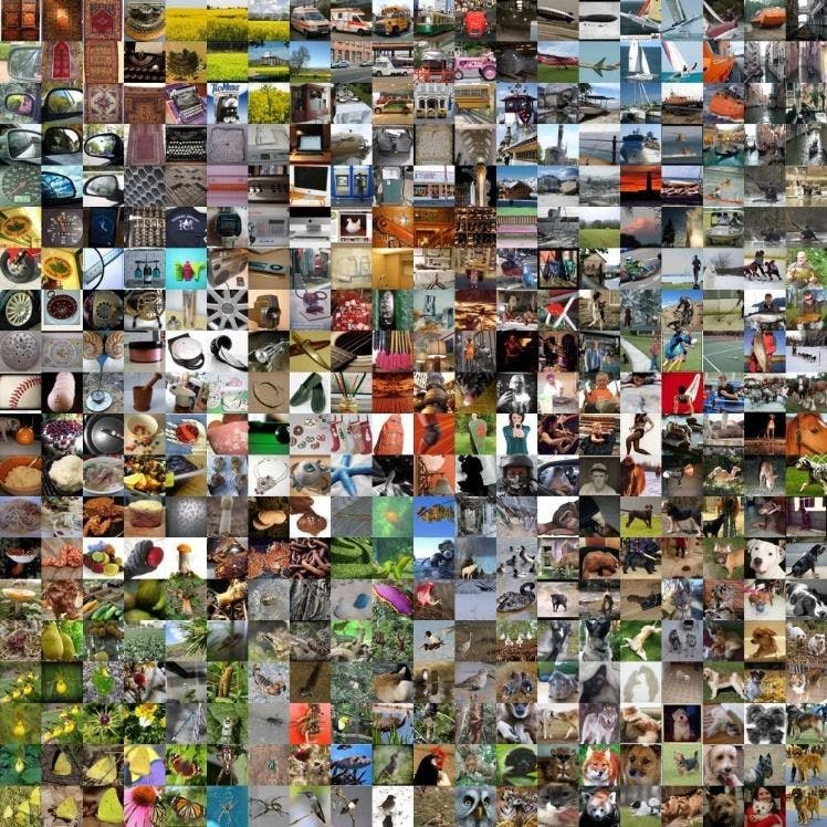
The list of all available models can be found on the Keras documentation page. They were trained on the ImageNet classification problem and can be used directly.

The accuracy of these models as well as the parameters they have used can be seen. The depth of the models are shown as well.
Here’s a look at the code.

Loading dataset

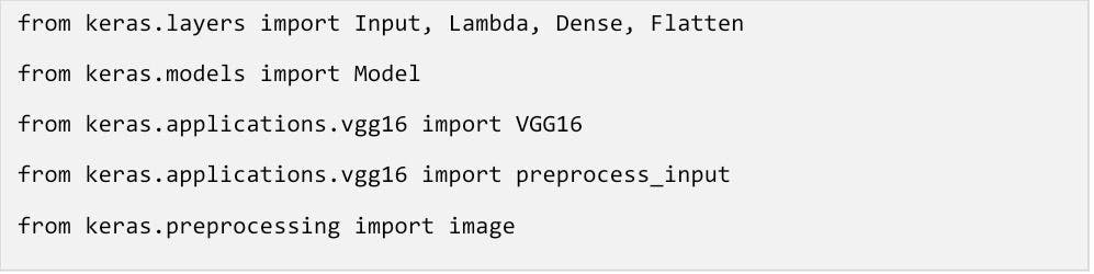
First, import the necessary libraries.

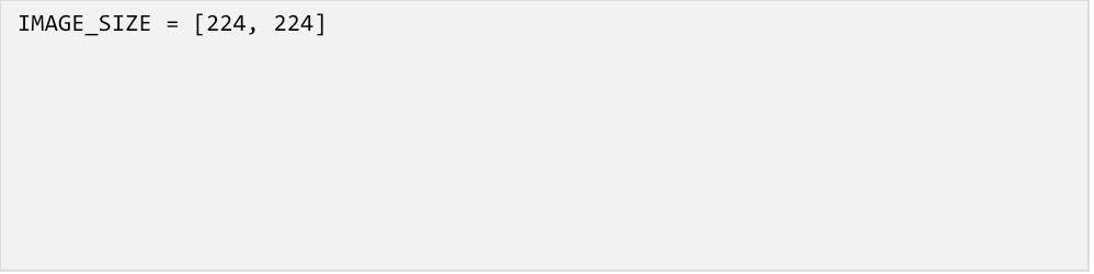
Next, mention the image size. Keep in mind that the model was trained on the ImageNet classification problem, so it may have a different input size. As the problem and the particular image could be of different sizes, you need to change the input layer.

The ImageNet classification problem has the output as 1000 classes, but you could have fewer as well. Know that you need to make a change in the output layer. All the hidden layers and all the convolution layers and weights of those layers remain the same.

For the purpose of demonstration, let’s use the skin cancer dataset, which contains a number of images classified as benign and malignant. The dataset can be downloaded here.

In the next step, specify the train path and the test path.

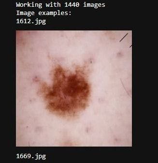
This next step, which is not compulsory, displays the benign images.

Output:

Output:

Implementing transfer learning

Now that the dataset has been loaded, it’s time to implement transfer learning.

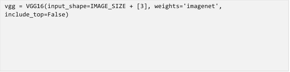
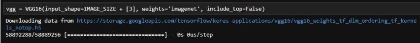
Begin by importing VGG16 from keras.applications and provide the input image size. Weights are directly imported from the ImageNet classification problem. When top=False, it means to discard the weights of the input layer and the output layer as you will use your own inputs and outputs.

Output:

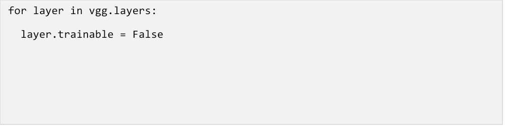
For layer in vgg.layers, layer.trainable=False to indicate that all the layers in the VGG16 model are not to be trained again. You only want to directly use this parameter.

Output:

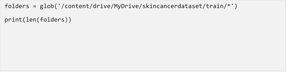
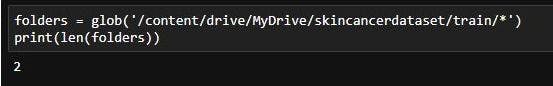
You can get the number of folders using glob.

Output:

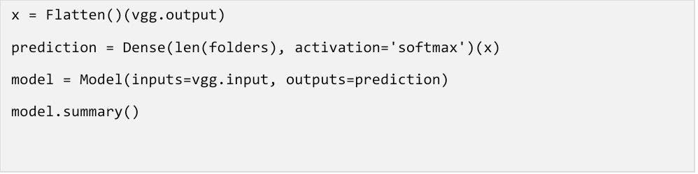
Next, specify a flatten layer so that whatever output you get in the last layer will be condensed into one dimension. You need an output layer with only two neurons. The activation function used is softmax. You can also use sigmoid as the output has only two classes, but this is the more generalized way.

Output:

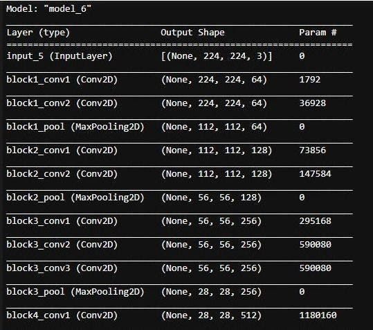
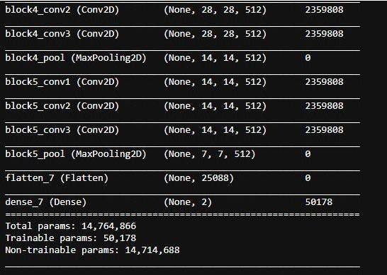
Now you can witness the magic of transfer learning. The total parameters are a massive 14 million but as you can see, the trainable parameters number only 15000. This reduces a huge amount of time and removes much of the complexity.

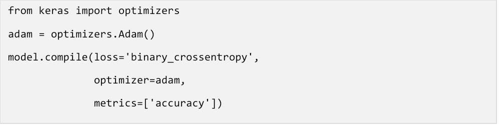
The following step experiments with Adam optimizer, binary_crossentropy loss function and accuracy as metrics.

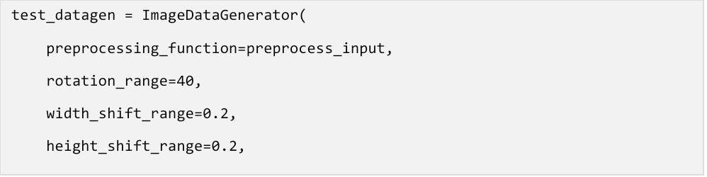
Data augmentation

The next stage is image augmentation. You will import prepocess_input as there were some preprocessing steps when the actual model was trained in the imagenet problem. To achieve similar results, you need to make sure that you use the exact preprocessing steps. Some, including shifting and zooming, are used to reduce overfitting.

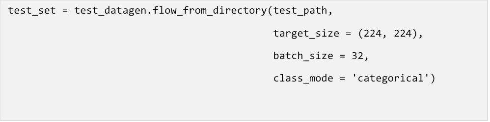
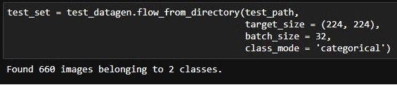
The same is done for the testing set.

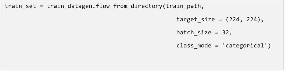
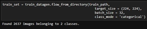
Specify the target size of the output, batch size, and the class.

Output:

The same is done for the testing set.

Output:

Training the model

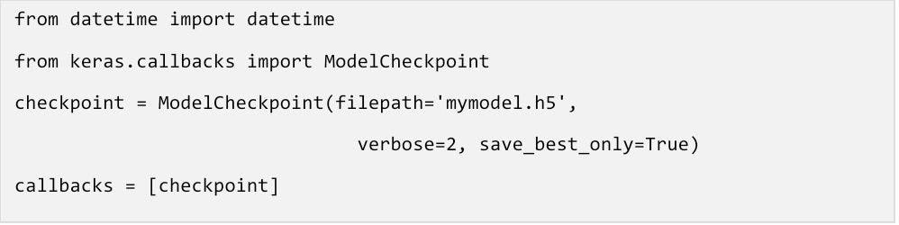
Now that data augmentation has been completed, it’s time to train the model. Model checkpoint is used to save the best model. You will use 10 epochs with 5 steps per epoch. The validation steps equal to 32.

Output:

Output:

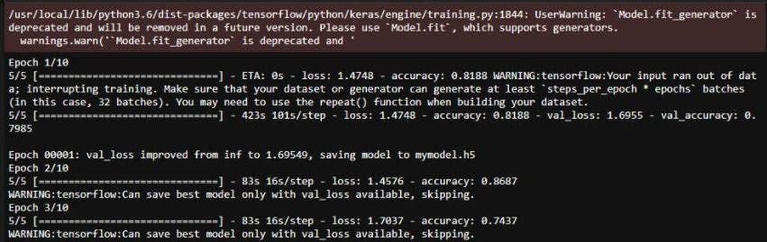
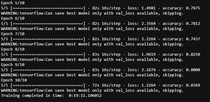
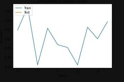
The accuracy can be seen once the training is done. The best part is that you don’t really have to do anything except to directly take the weights and develop the best performing model on the popular dataset.

Advantages of using transfer learning in machine learning

Among the many benefits of transfer learning, the top are:

• It saves time and resources. Most machine learning problems involve training a large amount of data. This type of labeled training data takes more time. However, in transfer learning most models are pre-trained, which reduces the size of training data.
• It improves the efficiency of a model while training. Developing machine learning models to solve complex problems is time-consuming. With transfer learning, you don’t need to create a model from scratch. You can reuse the developed model by transferring its knowledge.
• Instead of using different algorithms to solve new problems, transfer learning provides a more generalized way of solving the problem.

Applications of Transfer Learning

Here are some real-life applications of transfer learning.

• In natural language processing, transfer learning can be used to predict the next word in a sequence.
• Transfer learning models are well suited to recognize images. For example, a model developed to identify cats can be used to identify dogs.
• In speech recognition, the model developed to recognise one language can be used to recognise another language.
• The model developed to recognise MRI scans can be used to detect CT scans too.
• A machine learning model developed to classify emails can be used to scan spam mails.

As demonstrated, transfer learning is a very effective technique when working on image classification problems. Now that you’ve learned it using CNN, you can experiment with different models and perform hyperparameter tuning using Keras tuner.