How do you code for a binary image classification problem? How do you decide which loss function to use, and how do you code the architecture of a custom CNN model? This article will take you through these and more. By coding in Python, you will be able to detect pneumothorax (lung collapse due to air or gas in the cavity between the lungs and the chest wall) from an image of the chest X-ray scan of a patient. You will also gain insights on the challenges of deep learning in healthcare, the datasets with medical image modalities, and the role of image segmentation.

Dataset acquisition

The dataset for this exercise has been obtained from Kaggle. Download the zip file and extract it on your local system. You need the PNG images folder containing the chest X-ray images of healthy and pneumothorax-infected patients. You also need the two CSV files, stage1_train_images.csv and stage1_test_images.csv, for the train set and test set, respectively.

Note: Owing to the shortage of pneumothorax images in the original dataset, consider creating two copies of every pneumothorax image for training to balance the dataset.

Here comes the tricky part as you cannot directly access the images. They are not available category-wise in folders, which usually is the case with image classification on a custom dataset. The file names of the images - and whether it is a case of pneumothorax or not - have been recorded in the two CSV files. You need to code using this information in order to track the required images. You then need to store them in the folders to create the usual scenario of image classification on a custom dataset.

The final directory structure should be:

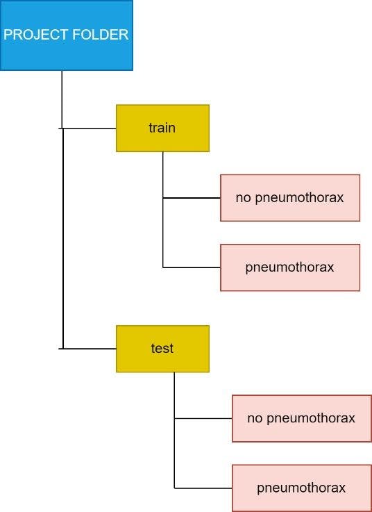
The different colors help track the folder levels.

As the dataset is very large, consider executing the project on your local system on Jupyter Notebook. You can also work on Google Colab but ensure that the underlying Google Drive has enough space to hold around 16,000 chest X-ray images.

Here starts the process. Begin with the train CSV file. Read it using the pandas' package like you would any other CSV file.

import pandas as pd

df=pd.read_csv("/content/drive/MyDrive/Pneumothorax
project/stage_1_train_images.csv")

0 means NO PNEUMOTHORAX and 1 means there is PNEUMOTHORAX. Now, get the list of the names of images that have and do not have pneumothorax.

no=list(df[df["has_pneumo"]==0]["new_filename"])

yes=list(df[df["has_pneumo"]==1]["new_filename"])

Decide where you want to store the images with and without pneumothorax as follows:

path="/content/drive/MyDrive/Pneumothorax project/png_images/"

img_path_no="/content/drive/MyDrive/Pneumothorax
project/train/no pneumothorax/"

img_path_yes="/content/drive/MyDrive/Pneumothorax
project/train/pneumothorax/"

The first path refers to where you have stored the PNG images downloaded from Kaggle. Use a package called shutil to move the images into the desired folder.

import shutil

The code below will move the healthy images from the PNG images folder to the no pneumothorax folder of the train folder.

for i in no:
src_path=path+i
dest_path=img_path_no+i
temp=shutil.move(src_path, dest_path)
print("No folder created and relevant images have been moved")

Move the pneumothorax images in a similar manner but to the pneumothorax folder instead of the no pneumothorax folder.

for i in yes:
src_path=path+i
dest_path=img_path_yes+i
temp=shutil.move(src_path, dest_path)
print ("Pneumothorax folder created and relevant images have been moved")

The same data acquisition steps can be followed to obtain the test dataset images from the test.csv file. The code is as follows:

df=pd.read_csv("/content/drive/MyDrive/Pneumothorax project/stage_1_test_images.csv")
no=list(df[df["has_pneumo"]==0]["new_filename"])
yes=list(df[df["has_pneumo"]==1]["new_filename"])
path="/content/drive/MyDrive/Pneumothorax project/png_images/"
img_path_no="/content/drive/MyDrive/Pneumothorax project/test/no pneumothorax/"
img_path_yes="/content/drive/MyDrive/Pneumothorax project/test/pneumothorax/"
for i in no:
src_path=path+i
dest_path=img_path_no+i
temp=shutil.move(src_path, dest_path)
print("No folder created and relevant images have been moved")
for i in yes:
src_path=path+i
dest_path=img_path_yes+i
temp=shutil.move(src_path, dest_path)
print("Pneumothorax folder created and relevant images have been moved")

This time, you will deal with the test folder instead of the train folder as you are acquiring the test dataset.

Data pre-processing

Import the required packages:

from tensorflow.keras.layers import Input, Lambda, Dense, Flatten,Dropout,Conv2D,MaxPooling2D,BatchNormalization
from tensorflow.keras.models import Model
from tensorflow.keras.preprocessing import image
from sklearn.metrics import accuracy_score,classification_report,confusion_matrix
from tensorflow.keras.preprocessing.image import ImageDataGenerator
from sklearn.model_selection import train_test_split
from tensorflow.keras.models import Sequential
import numpy as np
import pandas as pd
import os
import cv2
import matplotlib.pyplot as plt

Resize all the images to 50x50 (this image size can be anything).

re-size all the images to this

IMAGE_SIZE = (50,50)

The next step is to go through the images in the train and test folders, read them using OpenCV (cv2), get their array representations, and store them in the x_train and x_test lists. These are the features or inputs passed to the CNN model.

x_train=[]
x_test=[]
train_path="Pneumothorax project/train"
test_path="Pneumothorax project/test"

For train set:

c=0
for folder in os.listdir(train_path):
sub_path=train_path+"/"+folder
for img in os.listdir(sub_path):
image_path=sub_path+"/"+img
img_arr=cv2.imread(image_path)
try:
img_arr=cv2.resize(img_arr,IMAGE_SIZE)
x_train.append(img_arr)
except:
c+=1
continue
print("Number of images skipped= ",c)

For test set:

x_test=[]
c=0
for folder in os.listdir(test_path):
sub_path=test_path+"/"+folder
for img in os.listdir(sub_path):
image_path=sub_path+"/"+img
img_arr=cv2.imread(image_path)
try:
img_arr=cv2.resize(img_arr,IMAGE_SIZE)
x_test.append(img_arr)
except:
c+=1
continue
print("Number of images skipped= ",c)

Convert the lists to NumPy arrays and divide by 255, which is the normalization or major pre-processing step when handling image data.

x_test=np.array(x_test)
x_train=np.array(x_train)
x_train=x_train/255.0
x_test=x_test/255.0

Get the labels using ImageDataGenerator as follows:

datagen = ImageDataGenerator()
train_dataset = datagen.flow_from_directory(train_path,
class_mode = "binary")
test_dataset = datagen.flow_from_directory(test_path,
class_mode = "binary")

The labels are encoded with the code below:

train_dataset.class_indices

It will be 0 for no pneumothorax and 1 for pneumothorax in both the train and test datasets.
Assign these classes to y_train (training dataset"s labels) and y_test (testing dataset"s labels):

y_train=train_dataset.classes
y_test=test_dataset.classes

Confirm that the training data now has 15433 images and the test dataset has 1372 images.

x_train.shape,y_train.shape
x_test.shape,y_test.shape

(1372,50,50,3) indicates that there are 1372 images, each 50x50 (as they have been resized to this dimension), and 3 indicates that all of these are color images as taken from Kaggle.

Model building

This step will train the model with the features and labels obtained from the pre-processed images.
Build the model as follows:

model=Sequential()
Create a sequential model, which is a model that has one layer after another. It has input, followed by hidden and finally, the output layer.
Begin by adding convolution and pooling layers:

#convolution layer
model.add(Conv2D(64,(3,3),activation="relu",input_shape=(50,50,3)))
#pooling layer
model.add(MaxPooling2D(2,2))
model.add(BatchNormalization())
#convolution layer
model.add(Conv2D(128,(3,3),activation="relu"))
#pooling layer
model.add(MaxPooling2D(2,2))
model.add(BatchNormalization())
#convolution layer
model.add(Conv2D(256,(3,3),activation="relu"))
#pooling layer
model.add(MaxPooling2D(2,2))
model.add(BatchNormalization())

Three convolutional layers have been added along with batch normalization layers for better performance.
Add the input layer:

#i/p layer
model.add(Flatten())

Add the fully connected layer or final layer, i.e., the output layer:

#o/p layer
model.add(Dense(1,activation="sigmoid"))

Sigmoid function has been used as this is a binary classification problem. "1" indicates linear output. For multiclass problems, mention the number of categories instead of "1".
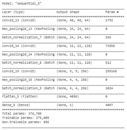
Here is a look at the custom model:

model.summary()

model.summary()

Compile the model with the right loss function:

#compile model:
model.compile(optimizer="adam",loss="binary_crossentropy",metrics=["accuracy"])

Binary cross entropy is the loss function used for binary classification. Use the best optimizer, "adam", as the learning rate is decided on its own and there is no need to mention the same. Avoid overfitting of the model using early stopping. It will stop training the model when the validation accuracy suddenly declines and the training accuracy increases.

from tensorflow.keras.callbacks import EarlyStopping
early_stop=EarlyStoppinga(monitor="val_loss",mode="min",verbose=1,patience=5)

Try training the model for 30 epochs:

history=model.fit(x_train,y_train,validation_data=(x_test,y_test),epochs=30,callbacks=[early_stop],shuffle=True)

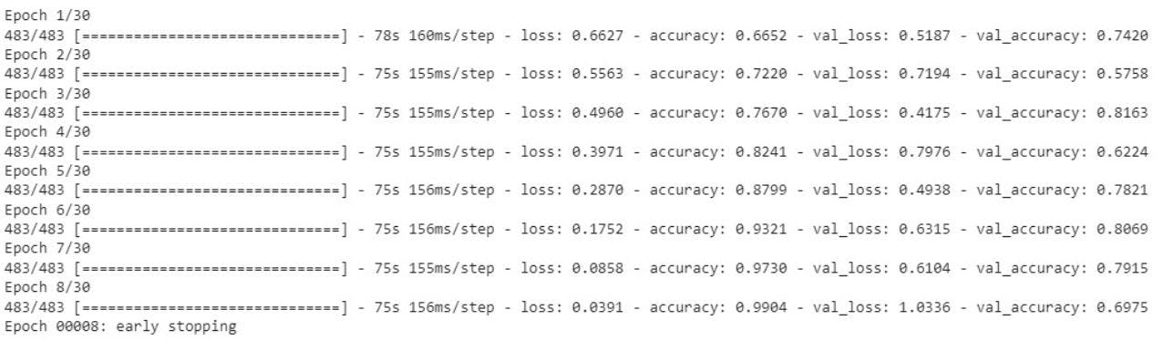
The training stops after 8 epochs to avoid overfitting just at the right time.

Results

The training accuracy is 99.04%. Test the model on the unseen data (test data) and use sklearn"s confusion matrix and classification report to evaluate it.

The loss and accuracy graphs of the model during the training are as follows:

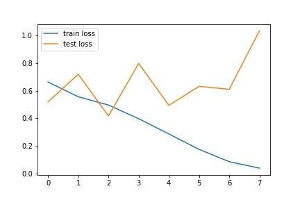
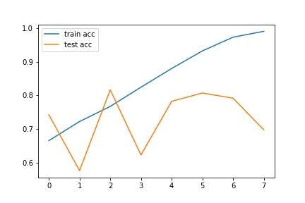
The above graphs show the gradual performance of the model with increasing epochs. Notice that there are several fluctuations in the test line, whereas the train accuracy increases and the train loss decreases with epochs.

Predict for all the samples in the test set:

y_pred=model.predict(x_test)
y_pred=np.argmax(y_pred,axis=1)

Get the accuracy score (VALIDATION ACCURACY) of the model:

accuracy_score(y_pred,y_test)

It comes out to 78.86%. The detailed performance can be seen using the classification report and confusion matrix with the code below:

print(classification_report(y_pred,y_test))

print(classification_report(y_pred,y_test))

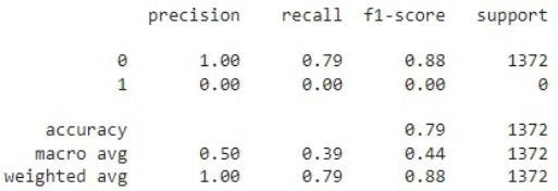
Thus, the validation accuracy is 79%. However, the model is able to recognize only non-pneumothorax images and is unable to detect pneumothorax on unseen or new images.

This can be inferred from the confusion matrix below:

confusion_matrix(y_pred,y_test)

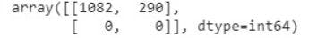
All the images are classified as non-pneumothorax.
The model always predicts the “no-pneumothorax” class for unseen samples. However, its performance is excellent with the training data. This may be because the train and test samples are not from the same spread, i.e., the test and train images were not taken from the same source of images. The test set has very different features compared to the train set. This can be a problem in most cases when the model exhibits poor performance on the test data.

The lack of distinct pneumothorax chest X-ray images may also be the cause. The problem with medical data is that you can find millions of healthy X-rays, CT scans, etc., but collecting the same for diseased patients is difficult. Pneumothorax is also rare.

Collecting patient samples involves many challenges, the topmost being patient privacy. Hospitals will not easily give out data. To improve the model, segmentation can be applied, which is the process of partitioning an image into several regions, depending on the similarity between adjacent pixels.

CNN extracts features from each and every pixel of the image. However, the intent here is to make it learn from only selected features, especially when it comes to medical images. For instance, in this problem statement, the aim is to get the model to extract features only from the part of the image between the lungs and the chest wall where pneumothorax infection occurs. This is why the zip file of the original dataset has masks in it.

Segmenting the chest X-ray images with the help of the masks, followed by using these masked images to train the CNN model, may help. Consider fine-tuning the model further or check with pre-trained architectures including VGG-19 or Mobile Net for the task.