Softmax Activation Function with Python
•4 min read
- Languages, frameworks, tools, and trends

The softmax activation function is one of the most popular terms we come across while resolving problems related to machine learning, or, more specifically, deep learning. We place softmax activation function at the end of a neural network in the deep learning model. Why? Because it normalizes the network output to a probability distribution over the estimated output classes.
We leverage this as an activation function to resolve multiclass classification problems. It can also be perceived as a generalization of the sigmoid function since it is used to present a probability distribution for a binary variable.
Note: If we look for softmax in the output layer in the Keras deep learning library with three-class classification activity, it might look like the example given below.
In order to implement it in Python, we will help you to briefly learn it from scratch. Let’s start with the mathematical expression for the same in Python.
Mathematical representation of softmax in Python
The softmax function scales logits/numbers into probabilities. The output of this function is a vector that offers probability for each probable outcome. It is represented mathematically as:
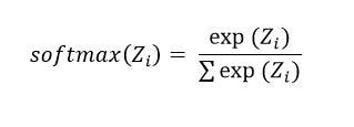
Where:
- Z = It is the input vector of the softmax activation function. It comprises n elements for n classes.
- Z(i) = It is i-th element of the input vector that takes up any value between negative infinity to positive infinity.
- exp [Z(i)] = It is the standard exponential function applied to Z(i). The resulting values may be tiny but they are never zero.
- n= It represents the number of classes
- Σexp [Z(i)] = It is a normalization term that makes sure the output vector value sums up to 1 for the i-th class.
Here’s an example to understand how it works as per this formula.
How softmax formula works
It works for a batch of inputs with a 2D array where n rows = n samples and n columns = n nodes. It can be implemented with the following code.
This is the simplest implementation of softmax in Python. Another way is the Jacobian technique. An example code is given below.
The above-mentioned Python code implementations are only pitched and tested for a batch of inputs. This means that the expected input is a 2D array with rows. It presents different samples and columns defining different nodes.
If you wish to speed up these implementations, use Numba which is best known for translating the subset of Python and NumPy code into fast machine code. To install it, use:
Note: Make sure that your NumPy is compatible with Numba, though pip takes care of the same most of the time.
Here’s how you can implement softmax NUMBA.
Here’s the code for the softmax derivative (Jacobian) NUMBA implementation.
Code source
These methods are quite fast with TensorFlow and PyTorch. However, there is another method that can be used to accelerate the implementation of softmax in Python. It is with the help of Cupy (CUDA) which is an open-source array library that is used for GPU-accelerated computing with Python.
Here’s what the Cupy implementation looks like:
Using these different methods, you can efficiently implement the softmax activation function in Python.
Example -
Assume a neural network that classifies an input image, whether it is of a dog, cat, tiger, or none.
Consider the feature vector to be X = [x1, x2, x3, x4]). In a neural network, the layout takes place as follows.
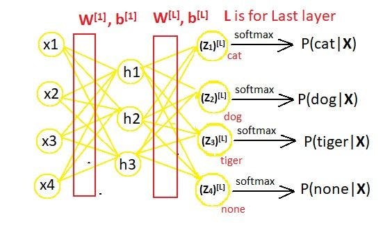
For the above-given neural network, the matrix will be:
![The vector Z [L] defined with its elements. (2).webp](https://images.prismic.io/turing/65a6af637a5e8b1120d59544_The_vector_Z_L_defined_with_its_elements_2_acd54be9ba.webp?auto=format,compress)
Where the weight matrix is:
![Weight matrix W [L] defined with its elements..webp](https://images.prismic.io/turing/65a6af647a5e8b1120d59545_Weight_matrix_W_L_defined_with_its_elements_90f605a945.webp?auto=format,compress)
Here,
m = Total number of nodes in layer L-1
n = Total number of nodes in output layer L.
For the above-given example, we have m=3 and n=4.
the following are the calculated values at layer L-1.
![H[L] matrix defined with its elements..webp](https://images.prismic.io/turing/65a6af657a5e8b1120d59546_H_L_matrix_defined_with_its_elements_c1680815c5.webp?auto=format,compress)
The bias matrix is:
![Bias matrix b[L] defined with its elements..webp](https://images.prismic.io/turing/65a6af667a5e8b1120d59547_Bias_matrix_b_L_defined_with_its_elements_18f4f5fa0d.webp?auto=format,compress)
If we calculate the exponential values of each element in the Z [L] matrix, we will have to calculate values for:
![Formula for exponential values of each element in the Z [L] matrix.webp](https://images.prismic.io/turing/65a6af677a5e8b1120d59548_Formula_for_exponential_values_of_each_element_in_the_Z_L_matrix_0bd55af25c.webp?auto=format,compress)
And also for:
![Formula for sum of all exponential values of each element in Z [L] matrix.webp](https://images.prismic.io/turing/65a6af687a5e8b1120d59549_Formula_for_sum_of_all_exponential_values_of_each_element_in_Z_L_matrix_8f9e60b9f7.webp?auto=format,compress)
Now, let’s consider the numeric values of each expression we listed above to drive output. Suppose we input the following values for the Z [L] matrix:
![Z[L] matrix defined with numeric values..webp](https://images.prismic.io/turing/65a6af697a5e8b1120d5954a_Z_L_matrix_defined_with_numeric_values_53ce232ca1.webp?auto=format,compress)
With this, the exponential values will be:
![Calculation for exponential values of each element in Z [L] matrix.webp](https://images.prismic.io/turing/65a6af6a7a5e8b1120d5954b_Calculation_for_exponential_values_of_each_element_in_Z_L_matrix_da0341ecfe.webp?auto=format,compress)
And,
![Sum of all exponential values of each element in the Z [L] matrix.webp](https://images.prismic.io/turing/65a6af6b7a5e8b1120d5954c_Sum_of_all_exponential_values_of_each_element_in_the_Z_L_matrix_a994678fa8.webp?auto=format,compress)
Thus, if we calculate the probability distribution as per the following formula,
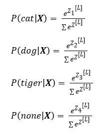
The probability distribution for the above example will result as:
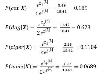
It is clear from the above values that the input image was that of a dog since it has a greater probability.
Implementing code for softmax function
If we have to implement a code for the above softmax function example in Python, here’s how it will be done.
Output of the code:
- Probability (Cat) = 0.19101770813831334
- Probability (Dog) = 0.627890718698843
- Probability (Tiger) = 0.11938650086860875
- Probability (None) = 0.061705072294234845
It clearly depicts that the input image is a dog as its output depicts the highest probability. This is the result we derived when we manually calculated the probability using the mathematical formula of the softmax activation function.
It’s time to get started!
This article sums up everything to get you started with implementing the softmax activation function in Python. From the multiple methods to speeding up the implementation using practical mathematical expressions and how they work behind the code - you have a clear understanding of all the resulting layers.