R Programming - How Is Maximum Likelihood Estimation Beneficial To Statistical Computing

Maximum Likelihood Estimation (MLE) in R programming is a method that determines the framework of the distribution of probability for the given array of data. Statistics, probability, and the ability to foresee outcomes are the keys to various sciences that we indulge in, it’s baffling just how much we leave to estimation.

With any large volume of data, the fastest and easiest way to comprehend the average is to simply get an estimation, and that is exactly what MLE does. It calculates the probability of occurrence of each of the data points for a given set of parameters in a model. MLE is a more structured and graphically semantic method.

In this article, we’ll take a look at Maximum Likelihood Estimation in R programming.

R programming language

R is a programming language that is engineered specifically for statistical computing including linear and non-linear modeling, time-series analysis, clustering, classification, and classical statistical tests.

One of the biggest strength of the R programming language is the ease it offers to produce a well-designed publication-level plot, which includes formulas and mathematical symbols. The user has complete control and this helps in progressing with the R programming language easily.

Now let’s take a look at some key benefits of maximum likelihood estimation in R programming environment.

Understanding probability & probability density in MLE

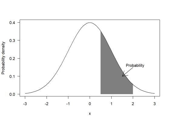
Let’s first understand probability and probability density in relation to continuous variables.

1. Probability density simply refers to the highest chance of a value or values occurring within a particular range on a data set. And unlike probability, probability density can process values that are greater than one.
2. Probability, on the other hand, is the selected range of the data set. It refers to the various values that might occur based on their probability density.

Keeping this in mind, let’s look at how MLE can help with estimations and probabilities to deliver an accurate result by understanding likelihood and the steps involved with calling the function.

Likelihood - what is it?

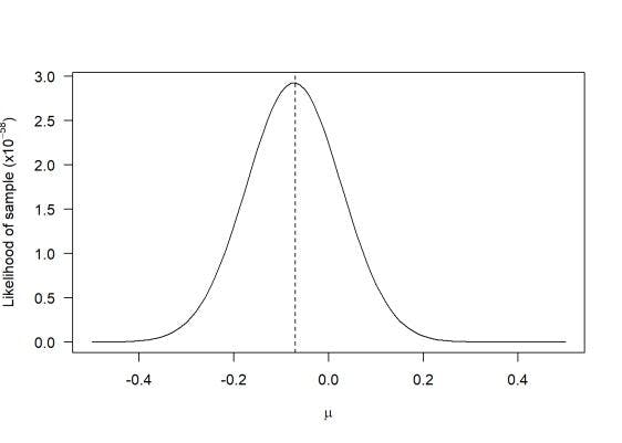
The ‘Likelihood Function’ is used to estimate the probability of certain events from a given data set. Each parameter specified in the parameter space is assigned a probabilistic prediction by the likelihood function based on the observed data.

Additionally, it usually incorporates data-generation processes along with missing-data mechanisms generated by the provided data set because the likelihood function is a realization of sampling densities.

When represented on a graph, we get something like this.

For example, if you try to estimate how many times a coin will land on heads or tails from a total of 10 flips, we would mostly assume a 50/50 chance of each landing. So in this case we would estimate 5 heads and 5 tails.

However, this method is never applicable in the real world where many variables exist. In these cases, we can use the ‘Likelihood Function’ to get far more accurate estimates pertaining to the available data set or sets.

But first there are two steps to be followed for MLE. Declaration and optimization, and we’ll be using the optim command for our optimization.

Declare the log-likelihood function

The maximum likelihood estimation in R programming generally take two arguments. One is that they require a vector of parameters and the other is requiring atleast one data set.

You can have additional arguments if required, but after arguments are declared they must be separated by { }.

The log-likelihood is expressed like this:

name<-function(pars,object){

declarations

logl<-loglikelihood function

return(-logl)

}

In the above code snippet, name is the log-likelihood function while pars is the name of the parameter vector and object is the name of the generic data object. Additionally, it’s important to ensure there are at least 2 elements.

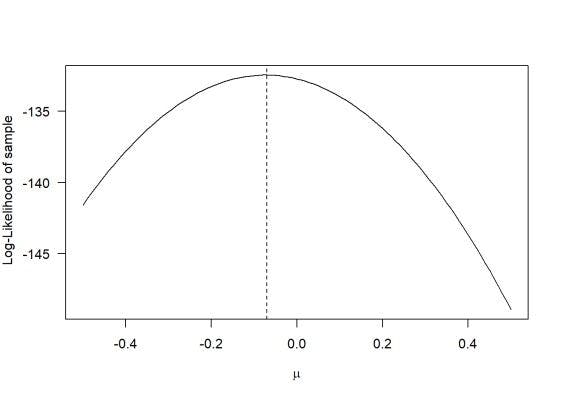
So when compared to the graph for likelihood above, we get something like this.

Image source

They are:

1. log1 - declaration of the log-likelihood function

2. return - return a value negative one times the log-likelihood.

You may also need to make other declarations such as temporary variables in the log-likelihood function or partitioning a parameter vector.

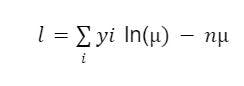
In this scenario, we’ll assume the Poisson log-likelihood function which is given in the equation below.

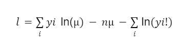
The last part of the equation does not contain the parameter μ, which means it can be ignored. This makes the equation as:

Now include it in the syntax:

poisson.lik<-function(mu,y){

n<-nrow(y)

return(-logl)

}

The next step is to optimize the log-likelihood.

Optimize the log-likelihood function

For this step, we are using theoptim command. You can use other optimization routines such as nlm or constr0ptim, but for now we’ll focus on the optim routine.

The base specification for optim is as follows:

optim(starting values, log-likelihood, data)

Now enter our starting values followed by the log-likelihood function we wish to use and finally declare the data and the end.

By default, the function utilizes the Nelder-Mead algorithm, however, you can change the algorithm by specifying method=”BFGS” to use the BFGS algorithm or method=”L-BFGS-B” to use the L-BFGS-B algorithm.

Let’s look at an example.

Assuming an unknown value to be in the MLE of poisson distribution. Now grab the estimates from the parameters by declaring the log-likelihood function poisson.lik.

Here, if we use the BFGS method, we end up with code like this:

optim(1,poisson.lik,y=data,method="BFGS")

In this instance, 1 is our starting value, and y refers to the generic data objects. It’s important to ensure the vector data is equated with y.

Finally, we move on to the output.

Final output

Since we used the optim function there are various pieces of output. This is true for other routines as well, but below are the general outputs you will get while using optim.

1. $par - It shows the maximum likelihood estimations for all parameters provided.
2. $value - It returns the log-likelihood times the number we requested which in this case is -1.
3. $counts - The number of calls to the log-likelihood function and the gradient are reported in this vector.
4. $convergence - It generally shows 0 indicating normal convergence, but if it shows 1 it will indicate that the iteration limit was exceeded. The default limit is 10000.
5. $message - Any errors during the optimization stage are shown here. If everything runs smoothly then the result should be NULL.

Let’s move on to the advantages of MLE for statistical computing.

Benefits of maximum likelihood estimation

It can be argued that other methods such as LSE (Least-square estimation) can be used successfully with zero error. But when it comes to estimating results from a large volume of data, MLE can’t be beaten.

Here’s why:

1. It is very easy to apply. Just call on the function and specify the method of estimation along with the parameters.
2. MLE is least affected by sampling errors that lower overall variance and the larger the sample size the lower the bias.
3. It’s a statistically significant and well-accepted method.
4. MLE is able to consistently provide approaches to parameter estimation issues because it has ability to analyze statistical models with varying characters on an equal basis,.
5. MLE can be developed for a massive number of estimation situations. Like if you have a huge volume of data, MLE can handle it easily.
6. Once MLE is derived, it provides statistical tests, errors, as well as other information that can be used for statistical interpretation later on.

There are many ways to estimate values from a given data set and other methods, in comparison, are more useful when it comes to smaller data sets. But MLE plays a huge role in estimating values for huge data sets.

Moreover, if you aren’t comfortable with the R programming language or other statistical computing languages, you can achieve the same or similar results on Python.

MLE Vs LSE

1. While there are a variety of estimation methods available, and in some cases, you might be benefitted from using estimators like LSE or Poisson regression, due to its unbiased nature it is far more reliable for real-world scenarios. While using methods such as LSE, the data set is locked to certain parameters which by default creates a biased estimation. MLE is also getting better with time as it is predominantly an unbiased method of estimation, and with enough information fed into the parameters, MLE can consistently provide accurate results.
2. MLE is especially useful when it comes to research centers and statistical analysis where large amounts of data are handled on a day-to-day basis. In theory, you can use LSE across various data sets to make assumptions till a proper estimate is calculated, which is definitely useful when working with limited data sets.
3. But even in this scenario, MLE comes out on top as this process of brute forcing with LSE is essentially MLE with unnecessary steps. It’s also because MLE leads in the Bayesian method very naturally. LSE, on the contrary, is a part of the bygone era. It is used today only because it was used extensively before. However, as with all things old, we need to move on and use faster and more efficient alternatives.

In simple terms, when it comes to quantitative disciplines and calculations, it’s far better to replace LSE with MLE.

While MLE can be used for any data sets including variables and multiple parameters, it is generally used to manage enormous amounts of data. Fortunately, MLE can be scaled up or down depending on the size of data provided and various parameters that are to be considered.

The information provided above can give you a basic understanding, however, there are many different methods, functions, and commands that can be used depending on the application. MLE in R programming can be extremely useful especially when you are managing and analyzing big data.

Frequently Asked Questions

What does maximum likelihood mean in statistics?

In statistics, maximum likelihood estimation (MLE) describes the process of estimating the parameters of an assumed probability distribution from the observed data.

What is the difference between MLE and MAP?

The MAP estimate will use more information than MLE does. Specifically, the MAP estimate considers both the probability and the prior knowledge of the system's condition.

Why is the maximum likelihood estimator a preferred estimator?

Parameter estimation problems can be addressed consistently with maximum likelihood. As a result, maximum likelihood estimations can be programmed for a wide range of estimation situations.

What is the difference between likelihood and probability?

Hypotheses are associated with likelihood; possible results are associated with probability.