How Machine Learning Can Be Used for Multiclass Classification in Python

Machine learning (ML) algorithms are used to classify tasks. They predict class categorization for a data point. It is the same way Gmail classifies email into spam/non-spam categories, Twitter segregates tweets into positive/negative/neutral sentiment, and Google Lens identifies the species of a plant from its image.

Types of multiclass classifications

Multiclass classification is broadly distinguished into:

1. Binary classification
2. Multiclass classification
3. Multi-label classification

Binary classification

When there are only two categories to classify data points, we refer to it as a binary classification. For example, detecting if a patient has tuberculosis (1) or not (0), or classifying whether a movie review is positive (1) or negative (0).

Multiclass classification

When the number of classes is more than two, it is referred to as multiclass classification.
For example, if we have to identify the digit in an image and classify it into any values between 0 and 0. For instance, we have 10 classes. We have to rate songs between 1 and 5 based on popularity. In these cases, each data point is allocated only a single class label.

Multi-label classification

There may be multiple labels predicted for single data input. For example, in the detection of objects from images, an image may have a house and a plant. This is called multi-label classification. All these types of classifications require a different approach and machine learning algorithms for prediction. Hence, it is important to identify what type of classification it is as a first step.

In this article, we will cover an in-depth analysis about multiclass classification in machine learning projects.

ML approaches for multiclass classification in Python

Multiclass classification is executed with machine learning, where algorithms are trained to learn patterns from structured labeled data. For simple binary classification, machine learning models like logistic regression and support vector machines (SVM) can be used.

While these models can handle only two classes, we can modify our multiclass classification as a problem of multiple binary classifiers and then use SVM. There are two different methods for implementing this: one-vs-all and one-vs-one.

These methods will be covered in the upcoming section. Apart from this, Naive Bayes classification, decision trees, and KNN ( K Nearest Neighbors) are the ML algorithms that can also be used. We’ll look into them too.

One-vs-all method

This is a simple method, where a multi-class classification problem with ‘n’ classes is split into ‘n’ binary classification problems. Let’s consider an example of classifying domestic animal images into 4 classes: dog, cat, cow, and pig.

To model this, we can build four individual binary classifiers for each class. The first classifier would predict if the image is a dog or not with some value of confidence. Similarly, the second classifier would predict if it is a cat or not, and so on.

In the end, we will choose the class for which the confidence value of prediction was highest. These individual binary classifiers could be logistic regression models. The sklearn library enables us to implement this easily.

To implement the models discussed above, we will generate a synthetic dataset using simple commands below. The "make_classification" function will generate a dataset with the inputs of our choice - features, classes, and how many samples we want.

from sklearn.datasets import make_classification        
x, y = make_classification(n_samples=3000, n_features=12, n_informative=5, n_redundant=5, n_classes=4, random_state=36)

Moving to the implementation of the one-vs-all method, we can use the logistic regression model of sklearn, with the ‘multi_class’ parameter set to ‘ovr’. Ovr is a short term for ‘one-vs-rest’ or ‘one-vs-all’, which informs the model on what strategy to adopt.

from sklearn.linear_model import LogisticRegression          
model = LogisticRegression(multi_class='ovr')       
model.fit(X, y)
predictions = model.predict(X)

The above code snippet shows how to fit the model and use it to make predictions on the dataset.

One-vs-one method

This is similar to the previous approach, except that here we train different binary classifiers for each class against each other (all unique combinations considered).

Take the same example of 4 domestic animal classes: dog, cat, cow, and pig. If we were to use this method, we would train 6 binary classifiers as shown below:

Classifier 1: Dog vs Cat
Classifier 2: Dog vs Cow
Classifier 3: Dog vs Pig
Classifier 4: Cat vs Cow
Classifier 5: Cat vs Pig
Classifier 6: Cow vs Pig

For a multiclass classification with ‘n’ classes, the number of binary classifier requisites would be n*(n-1)/2. Note that this method analyzes more models than the one-vs-all method. We can use logistic regression, SVM, KNN, and so on for the individual classifiers.

We can implement this using functions from the sklearn library’s multiclass module.

from sklearn.multiclass import OneVsOneClassifier
svc_model=SVC()   
ovo_model=OneVsOneClassifier(svc_model)
ovo_model.fit(x,y)

Now, let’s move on to some popular algorithms that usually work well on these types of problems. They can be used in company projects, Kaggle competitions, hackathons, and so on.

Decision tree classifiers

A decision tree is built by dividing a dataset into smaller subsegments based on certain conditions at each level. The idea is that every time a partition or division is made, similar data samples are grouped together.

The decision of how to split depends on entropy and information gained. Entropy refers to the randomness in the dataset, hence, the decision tree tries to make a split which will minimize the value of entropy of the data.

The initial nodes in a decision tree are the root nodes, and all the nodes, where splits are made, are called decision nodes. The final nodes at the end of the tree are the ‘leaf nodes’, which provide the prediction.

We will generate a dataset with 3 classes and train a decision tree classifier using the sklearn library.

x, y = make_classification(n_samples=500, n_features=5, n_informative=4, n_redundant=1, n_classes=3)              
X_train, X_test, y_train, y_test = train_test_split(X, y, test_size=0.3, random_state=1121218)

We can import the model from sklearn and use it as shown.

from sklearn.tree import DecisionTreeClassifier       
model = DecisionTreeClassifier()       
model.fit(X_train, y_train)             
y_pred = model.predict(X_test)

Now, we have the predictions of the model. We can generate a confusion matrix just like the binary classification to check the performance.

There will be minor differences in interpreting the confusion matrix for multiclass classification in Python compared to binary classifiers. The sklearn metrics module provides the necessary functions to implement this as shown below.

from sklearn.metrics import ConfusionMatrixDisplay, confusion_matrix
fig, ax = plt.subplots(figsize=(8, 5))   
cmp = ConfusionMatrixDisplay(confusion_matrix(y_test, y_pred),display_labels=["class_1", "class_2", "class_3"],)
cmp.plot(ax=ax)            
plt.show();

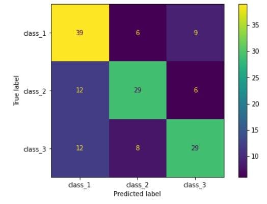
Here is the output obtained.

[Image source](Author’s Kaggle Notebook)

[Image source](Author’s Kaggle Notebook)

We can see that a 3 x 3 confusion matrix is generated. Looking at Row 1, we can see that out of the 54 total (39+6+9) data points of class 1, 39 of them were correctly predicted. 6 test points were misclassified into class 2 and 9 test points were misclassified as class 3. This is how we interpret the confusion matrix of multi-class classification problems.

Another major advantage is that we can actually plot and see how this decision tree derives the solution. We need to install the pydotplus package for this and then apply the “export_graphviz” function on the trained model as shown below.

!pip install pydotplus                
from sklearn import tree           
from IPython.display import Image, display              
import pydotplus            
dot_data = tree.export_graphviz(model, out_file=None,filled=True, rounded=True)            
graph = pydotplus.graph_from_dot_data(dot_data)            
display(Image(data=graph.create_png()))

[Image source](Author’s Kaggle Notebook)

[Image source](Author’s Kaggle Notebook)

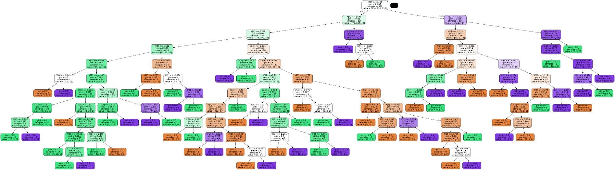
You can try this on different datasets like Iris and newsgroups to see how it works in each case.

Metrics to evaluate multiclass classification

In the previous section of the article, we learned how to use confusion matrix on multiclass classification problems. Now, we will take a look at other metrics as well.

In case of binary classification, precision, recall, and F1 score are the significant metrics calculated from the confusion matrix. The same principle is extended here to each class. For each class, we can separately calculate precision, recall, and F1 score.

To understand this better, we trained a model on a synthetic dataset with 4 classes. Below is the confusion matrix of it.

[Image source](Author’s Kaggle Notebook)

[Image source](Author’s Kaggle Notebook)

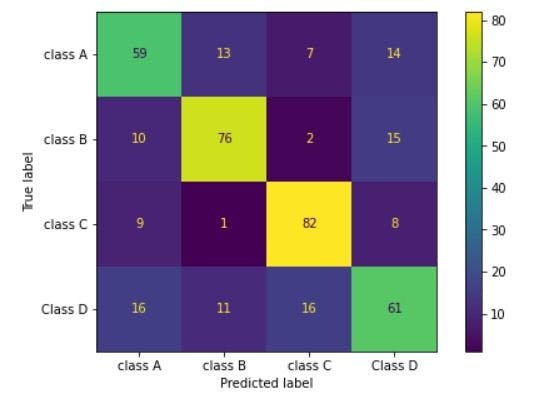
Let’s see how to calculate metrics for class A.

Total samples that belong to class A = 59 + 13 + 7+ 14 = 93
True positives (samples that belong to class A, was predicted as class A) = 59
False positives (samples that were classified as A, but do not belong to A) = 10 + 9 + 16 =35
Precision = True positives / (True positives + False positives)
Precision = 59/(59+35) = 0.627

That’s the mathematical explanation behind this. And though simple, it is essential. Sklearn provides an easy way to obtain these metrics for all classes using the “classification_report()” function.

from sklearn.metrics import classification_report
print(classification_report(y_test, y_pred))

[Image source](Author’s Kaggle Notebook)

[Image source](Author’s Kaggle Notebook)

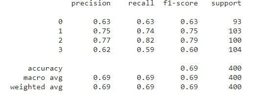
For class 0 or class A, we can verify that the precision value is the same as we had calculated with a small approximation.

In this article, we got to know what multiclass classification is, how it is different from binary classification, and how machine learning models can be applied to it. In this case, we used the decision tree classifier. Similarly, you can choose from a variety of options including random forests, XGBoost, LightGBM classifiers, etc.

These are ensemble methods that combine multiple decision trees for improved performance. When the dataset for multiclass classification contains images, you can also consider applying deep learning models with TensorFlow or PyTorch. Text classification models can be created similarly.