Data Collection and Data Preprocessing in Machine Learning with Python

Machine learning (ML) is an application of artificial intelligence (AI) that enables a computer or a system to learn and improve from experiences without being programmed explicitly. These experiences are nothing but patterns derived from past data. If you look at how the human brain works, it gains knowledge and insights from past experiences. ML also does the same thing. It relies on inputs called training data and learns from it. And what this means is that data is the most important aspect needed for an ML system to do its job.

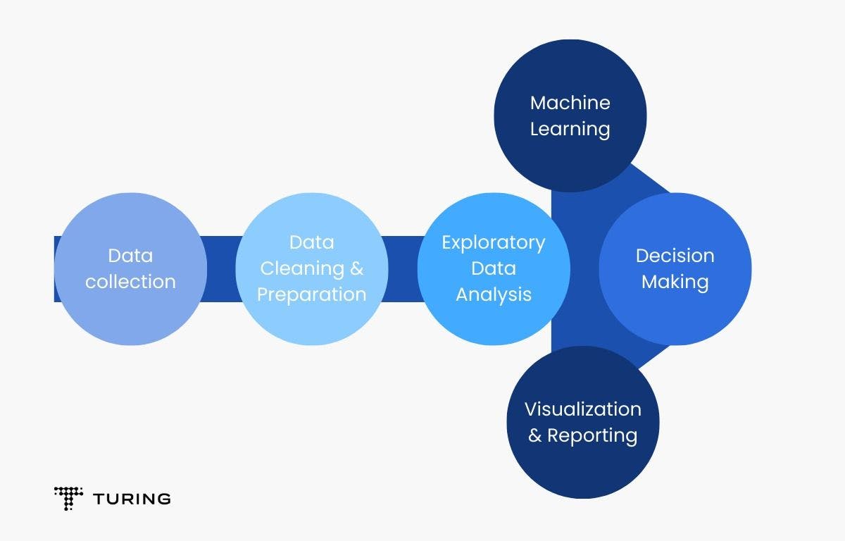
In the diagram above, it’s clear that data collection and data preparation are the foremost processes - and even the most significant - in the whole ML pipeline. This article will look at how they are vital for machine learning and how they can be done using Python.

Why is data collection important?

Simply put, without data, machine learning cannot exist. Data is what allows you to build predictive models using trends and insights harnessed from it. As records of past events are accumulated, patterns emerge and can be predicted over time.

Data collection for machine learning

Massive volumes of data are being generated each second via Google, Facebook, e-commerce websites, and more. While data is available in abundance, it has to be utilized in the best way possible.

Types of data

Many types of data are collected and used for machine learning. They can be in the form of text, tables, images, videos, etc. Some of the main types of data collected to feed a predictive model are categorical data, numerical data, time-series data, and text data.

Let’s look at them in detail.

1. Categorical data

In this type of data, an object is represented by different categories. Gender is an example of categorical data.

2. Numerical data

Also called quantitative data, this type is always collected in the form of numbers. For example, the number of girls and boys in different classes at a school.

3. Time series data

This data is obtained by repeated measurements over time. If you plot the graph for it, one axis will always represent time. Examples of time series data include temperature readings, stock exchange data, logs, weekly weather data, etc.

4. Text data

This data is text-based and may be in the form of articles, blogs, posts, etc. However, text data is converted into mathematical forms so computers can understand it.

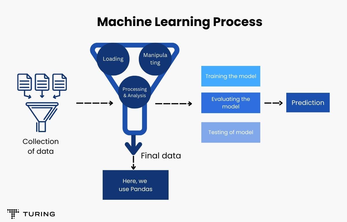
Once data is collected, it needs to be preprocessed before it’s fed to an ML model. Different feature engineering techniques can be used for the various types of features in data.

Data preprocessing using Python

Data preprocessing is nothing but preparing raw data in such a way that it can be fed to an ML algorithm. And in order to build a model, there are certain important steps that have to be followed:

1. Data collection
2. Data preparation
3. Choosing a model
4. Training
5. Evaluation
6. Parameter tuning
7. Prediction

Raw data that is collected in the data gathering stage is neither in the proper format nor in the cleanest form. It needs to undergo preprocessing steps such as:

• Splitting data into training, validation, and testing sets
• Handling missing values
• Dealing with outliers present in the data
• Taking care of categorical data/features
• Scaling and normalizing the dataset

Python libraries

Python provides a good set of libraries to perform data preprocessing. Here are a few important libraries.

1. Pandas

This is an open-source Python library built on top of NumPy. It’s mainly used for data clearing and analysis. It provides very fast and flexible data structures.

In the ML process of creating models and making predictions, Pandas is used right after the data collection stage. The library allows for several actions, including:

• Data cleansing
• Data fill
• Data normalization
• Data visualization
• Data inspection
• Merging and joining data frames
• Loading and saving data in various formats like CSV, Excel, HTML, JSON, etc.

Advantages of Pandas

• Provides functionality for loading data from different file objects
• Simplifies missing data handling
• Fast and efficient manipulation of data
• Provides time-series functionalities
• Enables efficient handling of huge data

2. Scikit-learn

Scikit-learn offers easy-to-use and effective tools for data processing in machine learning models. The commonly used processing tasks are OneHotEncoder, StandardScaler, MinMaxScaler, etc.

Here’s a quick look at the other preprocessing options in Sklearn.

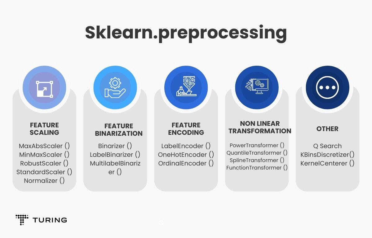
The Scikit-learn module also provides classification, regression, and clustering algorithms. It can easily be used to apply algorithms or for preprocessing tasks, owing to its well-written documentation.

Data preprocessing steps

Let’s take a look at some important data preprocessing steps performed with the help of Pandas and Sklearn.

1. Train-test split

Before data is fed to a model, it has to be split into various sets. Training data is given to a model to train it while validation and test data are used to perform validation and testing, respectively. The train and test split ratios are usually kept at 80:20, though this can vary depending upon the use case. Scikit-learn provides an in-built train-test split function.

Code:

from sklearn.model_selection import train_test_split                                  
X_train, X_test, y_train, y_test = train_test_split(X, y, test_size = 0.2)

2. Handling missing values

Raw data often contains missing values, garbage values, or NaN (not a number). It needs to be handled (made clean) before use in order to ensure better prediction results. Missing data can be filled with mean, mode, and median. To do this, the sklearn.impute module provides SimpleImputer, which can be used as:

from sklearn.impute import SimpleImputer
imputer = SimpleImputer(fill_value=np.nan, strategy='mean')
X = imputer.fit_transform(df)

This imputer returns the NumPy array, so it has to be converted back to dataframe.

X = pd.DataFrame(X, columns=df.columns)
print(X)

In many cases, it’s not possible to fill in missing data. Hence, these rows can be dropped using dropna in the Pandas module.

df_dropped=df.dropna()

3. Handling categorical features

Before data is used with categorical features, it has to be converted into integer form. There are two ways of doing this: label encoding and one-hot coding.

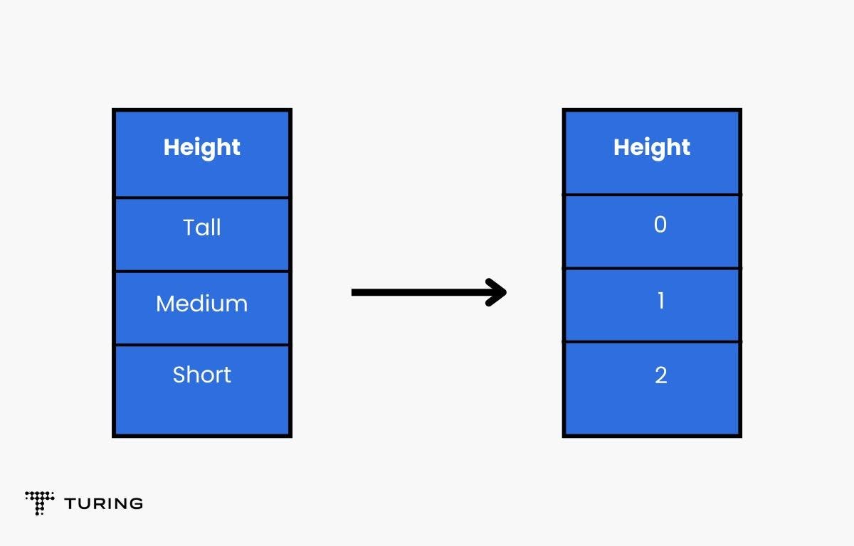
- Label encoding

Let’s take the example of a height column with Tall, Medium, and Short features. If you apply label encoding, the results will be: Tall as 0, Medium as 1, and Short as 2. This can be done via preprocessing modules imported from Sklearn.

Example:

from sklearn import preprocessing                                    
le = preprocessing.LabelEncoder()                                     
le.fit(["Tall", "medium",”medium”, "short"])                                          
le.transform(["Tall",”medium”, "short"])                   
list(le.inverse_transform([0, 1, 2]))                          

Output:

["Tall",”medium”, "short"]

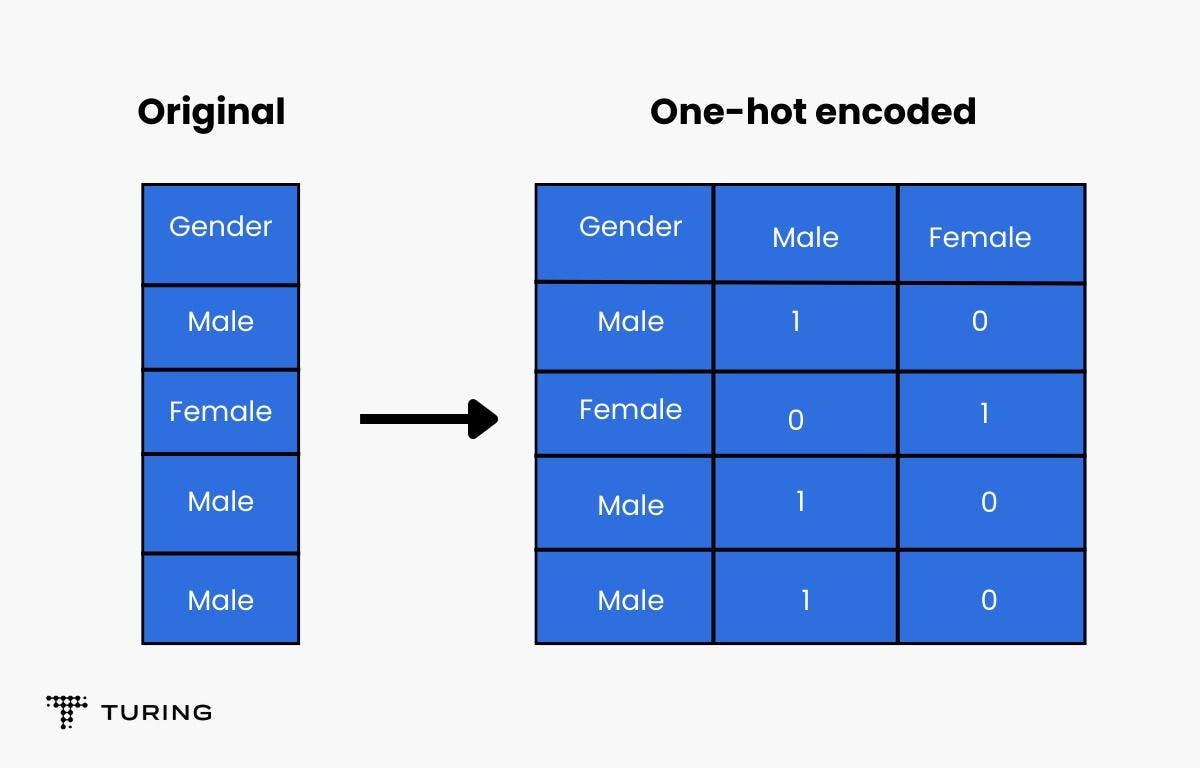
- One-hot encoding

This method encodes categorical features as a one-hot numeric array. It makes a separate column for all the categories in the categorical feature. For example, a gender column will have two values, male and female. One hot encoder will make one column for the male label and another for the female label. If the gender is male, 1 will be marked in the male column and 0 will be marked in the female column, or vice-versa.

The methods above are mainly used for numerical and categorical data. There are more advanced preprocessing steps as well.

Here’s a look at a few.

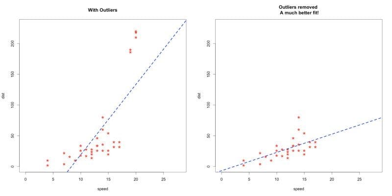
Handling outliers

Handling outliers is good practice before feeding data to a model as it makes it unbiased. Outliers are data points in a dataset that lie at an abnormal distance from others. Analysts decide what is considered abnormal. Depending on the distance, points can be categorized into mild outliers or extreme outliers. In most cases, extreme outliers are ignored and not used in modeling.

Image source

Using standard deviation in symmetric curve

If a symmetric curve has outliers present in a Gaussian distribution, you can set the boundary by taking standard deviation into consideration.

Using outlier insensitive algorithms

The easiest way to get rid of outliers is to use algorithms that are insensitive to outlier data points. For example, Naive Bayes classifier, support vector machine, decision tree, ensemble techniques, k-nearest neighbor, etc.

Data transformation

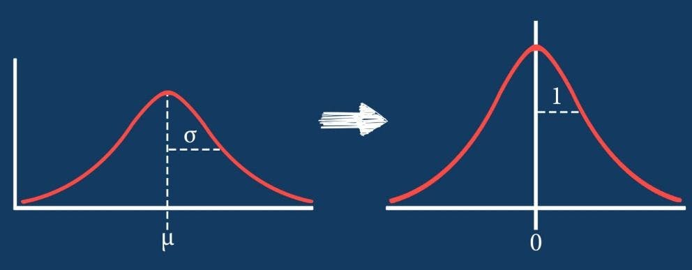
Datasets often contain features that differ a lot in magnitude, unit, and range. Directly feeding such data to a model without scaling it will result in poor modeling. This is because a model only takes magnitudes into account and not units. Hence, scaling must be done to bring all data to the same level. Standardization and normalization are two scaling techniques that can transform data.

- Standardization: The values are centered around the mean with a unit standard deviation. Hence, the mean of the attribute becomes zero and the resultant distribution has a unit standard deviation. The diagram below illustrates this.

- Normalization: In this scaling technique, values are shifted and rescaled to a range between 0 and 1. This technique is also known as min-max scaling.

Gaussian transformation

ML algorithms like linear and logistic regression assume that features are normally distributed. Hence, in these cases, certain transformation methods are used:

• Logarithmic transformation: uses logarithmic function, np.log(df[‘column_name’]
• Inverse transformation: uses inverse function, 1/(df[‘‘column_name’’])
• Square root transformation: uses square function, np.sqrt(df[‘‘column_name’’])
• Exponential transformation: uses an exponential function, df[‘‘column_name’’])**(1/1.2).

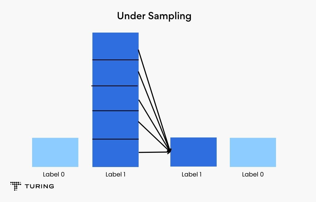
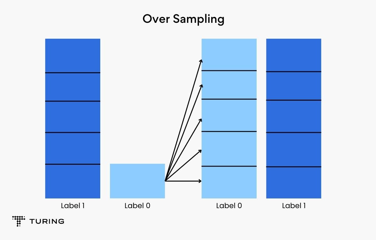
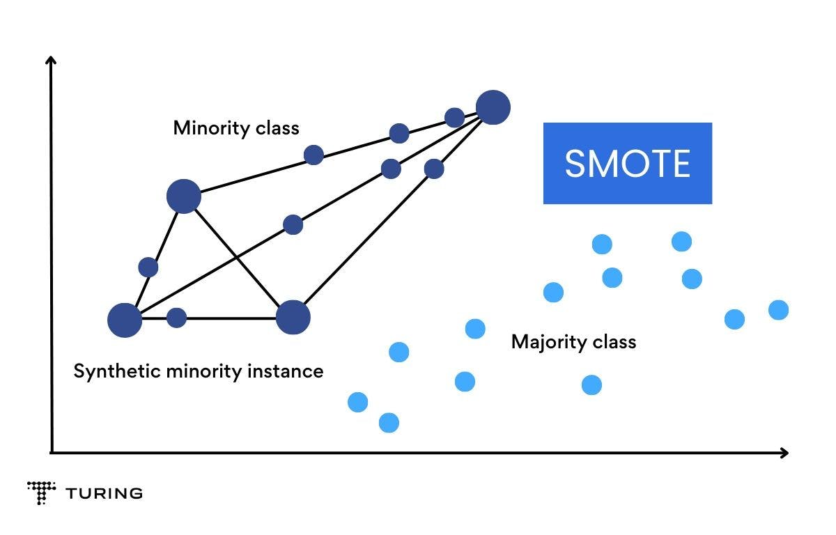
Handling imbalanced datasets

Balanced datasets are preferred as they improve accuracy and make a model unbiased. To do this, either the frequency of the minority class is increased or the frequency of the majority class is decreased. This provides approximately the same number of data points for all classes.

Here are a few resampling techniques.

- Under sampling: This technique works well when there are millions of data points. Here, some observations from the majority class are removed. This is done till the majority and minority classes are balanced out. The drawback is that when you remove data points, valuable information may also be removed which may hamper a model’s efficiency.

- Over sampling: More data points are added to the minority class in this technique. It works well when there isn’t a large chunk of data, but it can sometimes lead to overfitting.

- SMOTE: In Synthetic Minority Over-sampling Technique or SMOTE, synthetic data is generated for a minority class. It works by randomly picking a point from the minority class and finding the k-nearest neighbors for it. Synthetic points are added between these chosen points and the nearest neighbors.

Data that has to be preprocessed may not always be textual. It may be image data or time series data or other forms and so every type has to be preprocessed in a different way. But no matter the type, data collection and data preprocessing are two basic and very important steps in the entire machine learning pipeline. If skipped, an ML model will receive garbage data and yield garbage output. Hence, it’s vital to treat raw data.