A Step-By-Step Complete Guide to Principal Component Analysis | PCA for Beginners

Are you curious to learn about PCA? So, What exactly is a PCA?

You are lucky enough that you are at the right place! This guide will answer all of your questions.

PCA stands for Principal Component Analysis. It is one of the popular and unsupervised algorithms that has been used across several applications like data analysis, data compression, de-noising, reducing the dimension of data, and a lot more. PCA analysis helps you reduce or eliminate similar data in the line of comparison that does not even contribute a bit to decision-making. PCA analysis reduces dimensionality without any data loss. Yes! You heard that right. To learn more interesting stuff on PCA, continue reading this guide.

What is a PCA?

Principal Component Analysis finds the most common dimensions of the given data and makes result analysis better and easier.

Consider a scenario where you are dealing with a project that has significant variables and dimensions. Not all these variables will be critical. Some may be the primary key variables, whereas others are not. So, the Principal Component Method of factor analysis offers a calculative method to eliminate a few less important variables, thereby maintaining the transparency of all information.

Is this possible?

Yes, this is possible. PCA is thus called a dimensionality-reduction method. With reduced data and dimensions, you can easily explore and visualize the algorithms without wasting your valuable time.
Therefore, PCA statistics is the science of analyzing all the dimensions and reducing them as much as possible while preserving the exact information.

Where is PCA used in Machine Learning?

The Full form for PCA in Python and Machine Learning is the same as Principal Component Analysis with no more changes in meaning. These data concepts employ the same principle and technique. PCA statistics is the science of analyzing theories. You can find a few of its applications listed below.

You can find a few PCA applications in ML listed below:

1. PCA techniques aid data cleaning and data preprocessing techniques.
2. You can monitor multi-dimensional data (visualize in 2D or 3D) over any platform using the Principal Component Method of factor analysis.
3. PCA also helps in compressing the information and transmitting the same, using effective PCA analysis techniques. And all this information processing is done without any loss in quality.
4. This statistic is the science of analyzing different dimensions and can also be applied in several platforms like face recognition, image identification, pattern identification, and more.
5. PCA in ML techniques helps in simplifying complex business algorithms.
6. PCA minimizes the more significant variance of dimensions. You can easily denoise the information and completely omit the noise and external factors.

Principal Component Analysis example

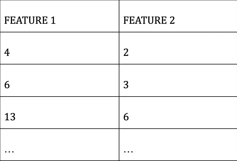
An example is taken for a demonstration to get a deep knowledge of PCA analysis. Imagine we have a dataset containing 2 different dimensions. Let the dimensions be FEATURE 1 and FEATURE 2, as tabulated below.

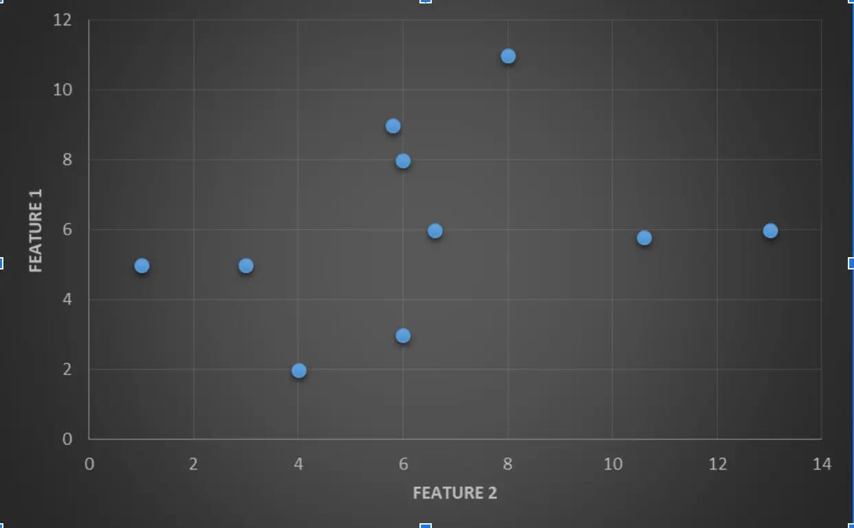
You can also represent the same dataset as a scatterplot, as depicted below. The two dimensions are listed along the X-axis (FEATURE 2) and Y-axis (FEATURE 1). You can find the datasets being distributed across the graph, and at some point, you may be clueless about how to segregate them easily. Here is some PCA analysis to help you out of the trouble.

Now, have a glance at the below graph. Here, two vector components are defined as FIRST PRINCIPAL COMPONENT and SECOND PRINCIPAL COMPONENT and computed based on a simple principle. The components that have a similar or greater amount of variance are grouped under a single category, and the components that have varying or smaller variances are grouped under the second category.

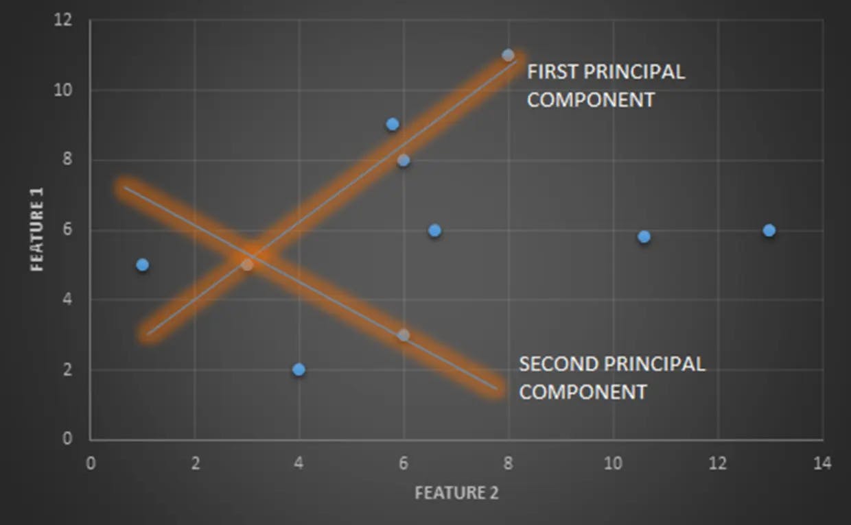
But always remember vectors calculated in the Principal Component Method of factor analysis are not calculated at random. All the calculated components can be combined as linear components, and so a single straight vector of each component helps you identify the difference in features much easier than ever.

Why is PCA useful?

In this guide, we have demonstrated a very small 2-dimensional example. You may doubt whether PCA in Machine Learning is really helpful. Please don’t wonder if we say Yes! What if you need to handle 100 variables?

Why not consider a real-time example?

Let's take a situation where you have to recognize a few patterns of good-quality apples in the Food processing industry. Do you think that the factory will only contain two digits or three-digit quantities? Definitely Not!

When you have to detect and recognize thousands of samples, you would require an algorithm to sort this out. Principal Component Analysis in Machine Learning helps you fix this problem.

As a first step, all possible features are categorized as vector components, and all the samples are passed out through an algorithm (simply like a sensor that scans the samples)for analysis.

After analyzing the bulk reports of the algorithm, you may categorize the apple samples with greater variances ( very small/ very large in size, rotten samples, damaged samples, etc.). At the same time, you may categorize other apple samples that have smaller variances like (samples with leaves or branches, etc., samples that are not under vector component values, etc.). So, now the samples that have greater variances will act as FIRST PRINCIPAL COMPONENT, and the samples that have smaller variances will act as SECOND PRINCIPAL COMPONENT.

When you represent these two Principal components over a pictorial representation in separate dimensions on the correct scale, you will get a clear view of the report. Also, the components out of the border can be considered additional ( noise) components and can be ignored if needed.

Now, you would have gathered a simple knowledge of the concept of Principal Component Analysis. This is just an example intended to give you a clear view of the process. Apart from this, there are a few other calculative steps involving calculating covariance matrix, defining eigenvalue, computing eigenvectors, and other statistical processes to give you more preservative information without losing any data. The next section will help you learn these processes.

Step-by-step explanation of PCA

In this section, you will learn about the steps involved in the PCA process.

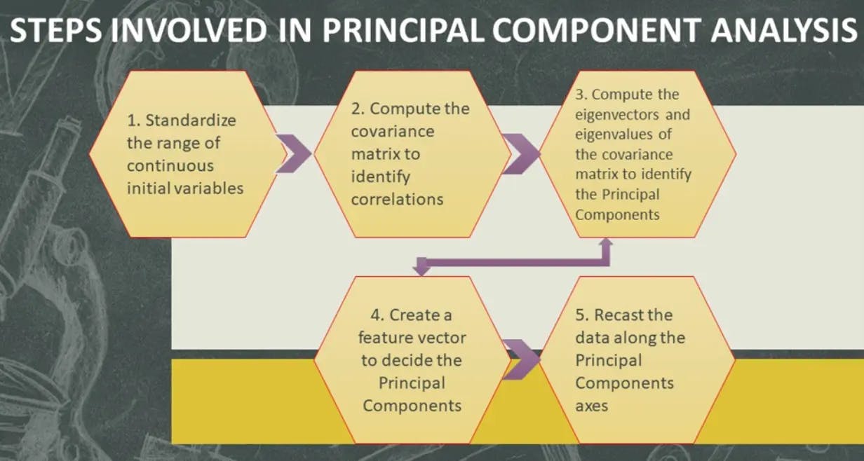
STEP 1: STANDARDIZATION

1. The range of variables is calculated and standardized in this process to analyze the contribution of each variable equally.
2. Calculating the initial variables will help you categorize the variables that are dominating the other variables of small ranges.
3. This will help you attain biased results at the end of the analysis.
4. To transform the variables of the same standard, you can follow the following formula.

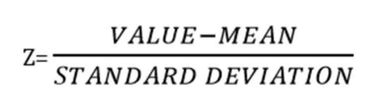
Where,

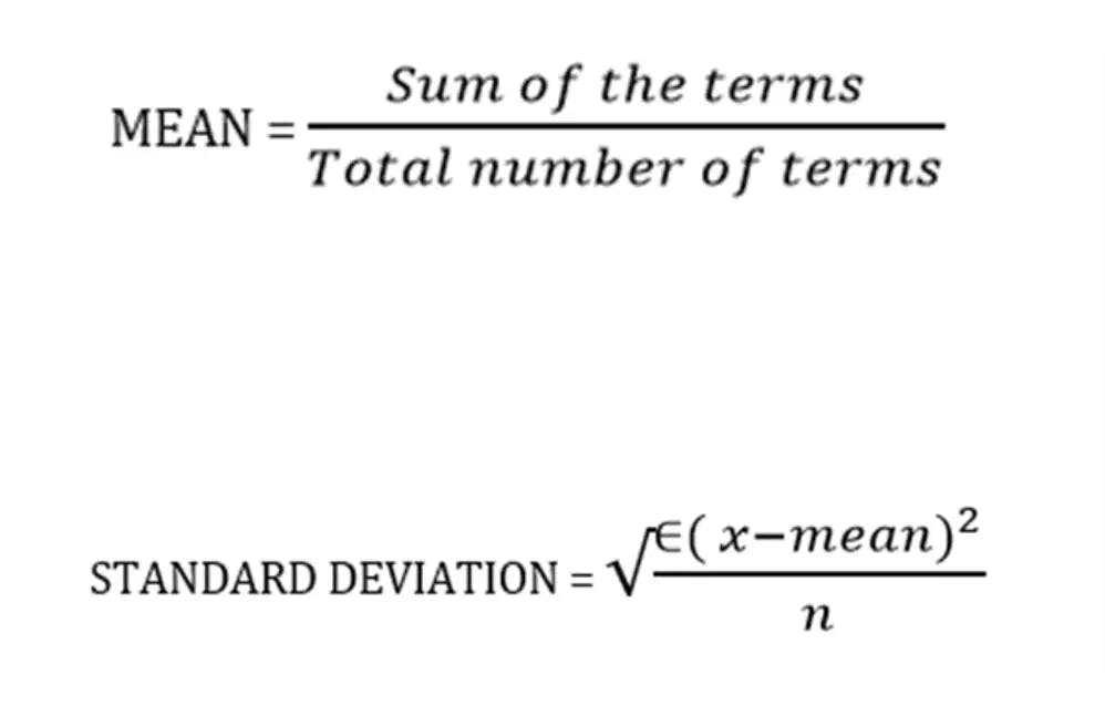
X= value in a data set

n= number of values in the data set

You can refer to the Standard Deviation Formula if you have any doubts about calculating Standard Deviation.

Example:

Let’s consider the same scenario that we have taken as an example previously. Let us assume the following features of dimensions as F1, F2, F3, and F4. Calculate the mean and standard deviation for each feature and then, tabulate the same as follows.

Then, after the standardization of each variable, the results are tabulated below.

This is the standardized data set.

STEP 2: COVARIANCE MATRIX COMPUTATION

1. In this step, you will get to know how the variables of the given data are varying with the mean value calculated.
2. Any interrelated variables can also be sorted out at the end of this step.
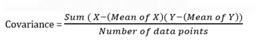
3. To segregate the highly interrelated variables, you calculate the covariance matrix with the help of the given formula.

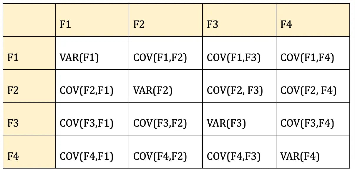
**Note: **A covariance matrix is a N x N symmetrical matrix that contains the covariances of all possible data sets.

The covariance matrix of two-dimensional data is, given as follows:

Where,

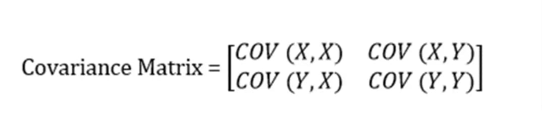
4. Make a note that, the covariance of a number with itself is its variance (COV(X, X)=Var(X)), the values at the top left and bottom right will have the variances of the same initial number.

5. Likewise, the entries of the Covariance Matrix at the main diagonal will be symmetric concerning the fact that covariance is commutative (COV(X, Y)=COV(Y, X)).

6A. If the value of the Covariance Matrix is positive, then it indicates that the variables are correlated. ( If X increases, Y also increases and vice versa)

6B. If the value of the Covariance Matrix is negative, then it indicates that the variables are inversely correlated. ( If X increases, Y also decreases and vice versa).

7. As a result, at the end of this step, you will come to know which pair of variables are correlated with each other, so that you might categorize them much easier.

Example:

So, continuing with the same example,

The formula to calculate the covariance matrix of the given example will be:

Since you have already standardized the features, you can consider Mean = 0 and Standard Deviation=1 for each feature.

var(F1) = ((-1.0-0)² + (0.33-0)² + (-1.0-0)² +(0.33–0)² +(1.33–0)²)/5

On solving the equation, you get var (F1) = 0.8

cov(F1,F2) =
((-1.0–0)(-0.632456-0) +
(0.33–0)(1.264911-0) +
(-1.0–0)* (0.632456-0)+
(0.33–0)(0.000000 -0)+
(1.33–0)(-1.264911–0))/5

On solving the equation, you get cov(F1,F2) = -0.25298

Similarly solving all the features, the covariance matrix will be,

STEP 3: DEFINE EIGENVALUE AND EIGENVECTOR

1. To determine the principal components of variables, you must define eigenvalue and eigenvectors for the same.
Let A be any square matrix. A non-zero vector v is an eigenvector of A if

Av = λv

for some number λ, called the corresponding eigenvalue.

2. Once you have computed the eigenvector components, define eigenvalues in descending order ( for all variables), and now you will get a list of principal components.

3. So, the eigenvalues represent the principal components, and these components represent the direction of data.

4. This indicates that if the line contains large variables of large variances, there are many data points on the line. Thus, there is more information on the line too.

5. Finally, these principal components form a line of new axes for easier evaluation of data, and also the differences between the observations can also be easily monitored.

Example:

Let ν be a non-zero vector and λ a scalar.

As per the rule,

Aν = λν, then λ is called the eigenvalue associated with eigenvector ν of A.

Upon substituting the values in det(A- λI) = 0, you will get the following matrix.

When you solve the following matrix by considering 0 on the right-hand side, you can define eigenvalues as

λ = 2.51579324, 1.0652885, 0.39388704, 0.02503121

Then, substitute each eigenvalue in the (A-λI)ν=0 equation and solve the same for different eigenvectors v1, v2, v3, and v4.

For instance,

For λ = 2.51579324, solving the above equation using Cramer's rule, the values for the v vector are:
v1 = 0.16195986
v2 = -0.52404813
v3 = -0.58589647
v4 = -0.59654663

Follow the same process, and you will form the following matrix using the eigenvectors calculated as instructed.

Now, calculate the sum of each Eigen column, arrange them in descending order, and pick up the topmost eigenvalues. These are your principal components.

STEP 4: FEATURE VECTOR

1. In this step, you will decide whether to keep or discard the variables of low eigenvalues for consideration.
2. Thus, the remaining set of eigenvalues will form a matrix of vectors called a Feature vector.
3. This Feature vector only contains the eigenvector columns that have significant importance of dimensionality.
4. If you keep only M eigenvector components out of N, the final data set will only have M components. Remember, there will not be any huge information loss.
5. As you have already found the total significance of each eigenvalue in the previous step, in this step, just pick the columns containing the topmost eigenvalues.

Example:

Now, calculate the sum of each Eigen column, arrange them in descending order, and pick up the topmost eigenvalues.

These are your principal components (feature vector matrix) in your PCA analysis.

STEP 5: RECAST THE DATA ALONG THE PRINCIPAL COMPONENTS AXES

1. Apart from standardization, you haven’t changed the original data. You have just selected the Principal components and formed a feature vector. Yet, the initial data remains the same on their original axes.
2. This step aims to reorientate data from their original axes to the ones you have calculated from the Principal components.

The following formula can do this.

Final Data Set= Standardized Original Data Set * FeatureVector

Example:

So, in our guide, the final dataset becomes

By solving the above equations, you will get the transformed data as follows.

Did you notice something? Your large dataset is now compressed into a small dataset without any data loss! This is the significance of Principal Component Analysis.

Applications of PCA Analysis

1. PCA Machine Learning is used to visualize multidimensional data.
2. To reduce the dimensional data in healthcare data.
3. PCA Python helps to resize an image.
4. PCA is used to analyze stock data and forecasting data.
5. You can also use Principal Component Analysis to analyze patterns when dealing with high-dimensional data sets.

Advantages of PCA

1. Easy to calculate and compute.
2. Speeds up machine learning computing processes and algorithms.
3. Prevents predictive algorithms from data overfitting issues.
4. Increases performance of ML algorithms by eliminating unnecessary correlated variables.
5. Principal Component Analysis results in high variance and increases visualization.
6. Helps reduce noise that cannot be ignored automatically.

Disadvantages of PCA

1. Sometimes, PCA Python is difficult to interpret. In rare cases, you may feel difficult to identify the most important features even after computing the principal components.
2. You may face some difficulties in calculating the covariances and covariance matrices.
3. Standardization of data is an important step in PCA analysis and it cannot be ignored at all.
4. Sometimes, the computed principal components can be more difficult to read rather than the original set of components.

To wrap up…

So, that’s all about PCA. We hope we have covered enough content on Principal Component Analysis with an example in addition to step-by-step procedures. Please share your thoughts on Principal Component Analysis in Machine Learning or if you have any suggestions or comments regarding this guide, we would love to hear from you!