Know all About Upper Confidence Bound Algorithm in Reinforcement Learning
•7 min read
- Languages, frameworks, tools, and trends

Have you tried a slot machine and won amazing rewards? You may have noticed that luck sometimes favors you while at other times, you win a few cents or lose entirely. Have you ever wondered how to find the ‘lucky machine’ that rewards you with plenty of money? This problem is known as the multi-armed bandit problem and the optimal approach employed to solve it is UCB or upper confidence bound algorithm.
This article will detail what the multi-armed bandit problem is, UCB, the math behind it, and its research applications. A prerequisite is a basic understanding of reinforcement learning including concepts such as agent, environment, policy, action, state and reward.
Exploration-exploitation trade-off
When deciding what state it should choose next, an agent faces a trade-off between exploration and exploitation. Exploration involves choosing new states that the agent hasn’t chosen or has chosen fewer times till then. Exploitation involves making a decision regarding the next state from its experiences so far.
At a given timestep, should the agent make a decision based on exploration or exploitation? This is the trade-off. The concept is the foundation for solving the multi-armed bandit problem, or for that matter, any problem to be solved using reinforcement learning.
Multi-armed bandit
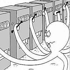
Consider the bandits or machines at a casino that you can pull with a trigger and win rewards. The above picture is a simple illustration to visualize the game. Whenever you pull one of the machines by its handle, you either win or lose. Note that you play with only one machine at a time.
Correlating the problem to reinforcement learning, the player is the agent here. Assume that different machines have different properties although this isn’t the case in real-life. In this case, one machine may give very good rewards while another may not.
How do you know which machine is the best? This is important for a player as the aim is to maximize the reward. You can find this out by playing with every bandit in the casino. As illustrated in the above picture, a player has multiple arms playing with multiple machines, indicating that the agent should play with all the machines. This enables the agent to learn about the machine’s properties.

An application of multi-armed bandit includes clinical trials. Since all drug versions can’t be tested, the optimal one should, thus, be tested.
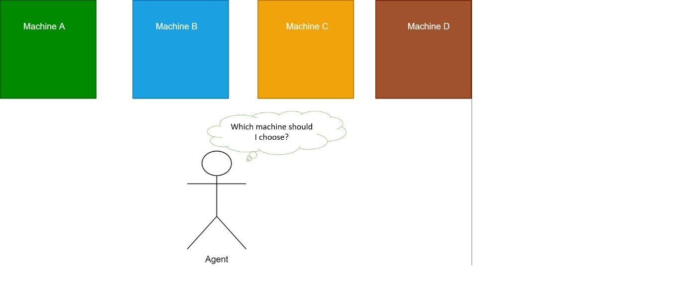
Image source: Author
Consider that there are four machines: A, B, C and D. The agent randomly chooses them and plays. The results are:
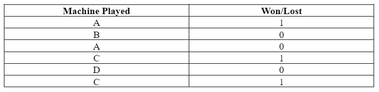
In the table above, the agent played with A and won. Exploring, the agent played with B and lost. Exploiting, it again played with A as it had won before. However, it lost. Exploring, it played with a new machine, C, and won. Exploring again, it played with a new machine, D, and lost. Exploiting, it returned to C but lost again. This process continues and is repeated until the agent maximizes its reward.
The math behind multi-armed bandit
Let the number of machines/bandits=n
Each machine i returns rewards yi which is approximately equal to P (y; θ_i)
Where θ_i is the probability distribution parameter. The machine provides rewards based on probabilities. The goal is to maximize the reward.
Introduction to UCB
Let’s formulate the multi-armed bandit’s problem this way:
Let t = current timestep
a_t is the decision or action taken by the agent at timestep t(action here refers to choosing one of the n machines and playing)
For instance, a_1 means action taken at timestep t=1
y_t is the reward or outcome at timestep t
policy π: [(a_1, y_1), (a_2, y_2)…….(a_(t-1),y_(t-1))] -> a_t
Policy maps everything the agent has learned so far to the new decision. This is why timesteps from t=1 to t-1 have been considered here.
Problem:
Find policy π that
<u>Case-1</u>: max

or
<u>Case-2</u>: max

<u>Case-1</u> finds a policy that maximizes the sum of all the rewards (as you can infer from the ∑ symbol).
<u>Case-2</u> finds a policy to maximize the reward obtained in the final step alone.
In case-2, agents need not care about intermediate rewards as the goal is to optimize only the final reward. Thus, in case-2, agents can explore and learn as much as possible. However, in case-1, the agent must collect as many rewards as possible.
So, which case should be chosen? This is where UCB algorithm comes in.
UCB1 algorithm
Ignore the 1 here.
Step-1: Initialization
Play each machine once to have minimum knowledge of each machine and to avoid calculating ln0 in the formula in step-2.
Step-2: Repeat
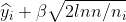
Play the machine i that maximizes
Until
END
Look at what is maximized in step-2.

= average reward of machine i so far

=how often machine i has been played so far
n=∑
=total number of rounds played so far
β is taken as 1(β=0.99, approximately considered as 1 mostly)
The first term,
, is the exploitative case. Here, the agent won’t learn much about the other machines. The second term

is the explorative case. It reduces entropy because, unlike the first term, it allows the agent to play with the less chosen machines so that you can better estimate if the current best machine is indeed the best.
Example problem for UCB1
Let’s understand the UCB algorithm with the help of an example.
Consider that there are three bandits being played and their corresponding rewards are as follows:
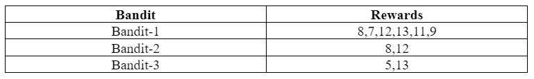
Question:
At the last timestep, which bandit should the player play to maximize their reward?
Solution:
The UCB algorithm can be applied as follows:
Total number of rounds played so far(n)=No. of times Bandit-1 was played + No. of times Bandit-2 was played + No. of times Bandit-3 was played.
So, n=6+2+2=10=>n=10
For Bandit-1,
It has been played 6 times. So,
= 6

= 8+7+12+13+11+9)/6=10
= 0.876
So, the value of step-2 is approximately 10.876.
For Bandit-2,
It has been played 2 times. So,
= 2
= (8+12)/2=10
=1.517
So, the value of step-2 is approximately 11.517.
For Bandit-3,
It has been played 2 times. So,
= (5+13)/2=9
= 1.517
So, the value of step-2 is approximately 10.517.
Time t is the last timestep. There won’t be any further exploration, so check where exploitation is maximum.
Bandit-1 and Bandit-2 have the same and the highest exploitation value (10). Which to choose? Considering entropy, it is Bandit-1 as it was played a greater number of times compared to Bandit-2. As it has less entropy, its value is more likely to be correct and is more expressive.
Hence, at the last timestep, the agent should play Bandit-1.
Let’s look at the two types of UCB-1 algorithms: UCB-1 Tuned and UCB-1 normal. These variations are obtained by changing the C value. The term under the square root in step-2 of the UCB1 algorithm is called ‘C’.
UCB-1 Tuned
For UCB1-Tuned,
C = √( (logN / n) x min(1/4, V(n)) )
where V(n) is an upper confidence bound on the variance of the bandit, i.e.
V(n) = Σ(x_i² / n) - (Σ x_i / n)² + √(2log(N) / n)
and x_i are the rewards gained from the bandit so far.
UCB1-Tuned is known to have outperformed UCB1.
UCB1-Normal
The term ‘normal’ in the name of the algorithm refers to normal distribution.
The UC1-Normal algorithm is designed for rewards from normal distributions.
The value of C, in UCB1-Normal, is based on the sample variance.
C = √( 16 SV(n) log(N - 1) / n )
where the sample variance is
SV(n) = ( Σ x_i² - n (Σ x_i / n)² ) / (n - 1)
x_i are the rewards the agent got from the bandit so far.
Note that to calculate C, each machine or bandit must be played a minimum of two times by the player to avoid division by zero. Each bandit is played twice as an initialization step. At each round N, it checks if there’s a bandit that has played less than the ceiling of 8logN. If it finds any, the player plays that bandit.
Research applications of UCB algorithm
Researchers have proposed strategies based on UCB to maximize energy efficiency, minimize delay, and develop network routing algorithms to optimize throughput and delay. A recent research project includes route and power optimization for Software Defined Networking (SDN)-enabled IIoT (Industrial IoT) in a smart grid, keeping EMI (electromagnetic interference) coming from the electrical devices in the grid.