Gradient Descent: An Optimization Technique in Machine Learning

In machine learning (ML), a gradient is a vector that gives the direction of the steepest ascent of the loss function. Gradient descent is an optimization algorithm that is used to train complex machine learning and deep learning models. The cost function within gradient descent measures the accuracy for each iteration of the updates of the parameter. The machine learning model continues to update its parameters until the cost function comes close to zero.

The gradient descent algorithm works iteratively in two steps:

1. Calculate the gradient that is the first-order derivative of the function at that point.
2. Move towards the direction opposite to that of the gradient.

Learning rate

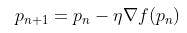
The gradient is multiplied by another parameter known as the learning rate and then subtracted from the current position to obtain the minimum of the function. The learning rate parameter significantly affects the performance of the model. For smaller learning rates, the model may reach the maximum iteration before reaching the optimal point, whereas it may not converge or may diverge completely if the learning rate is set large enough.

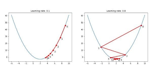
The above image shows that for a smaller learning rate (left), the model converges very slowly but more efficiently as compared to the case with a larger learning rate (right). Therefore, choosing an optimized value of the learning rate is crucial to get a model with the best accuracy.

Types of gradient descent

The gradient descent algorithm can be performed in three ways. They can be used depending on the size of the data and to trade-off between the model’s time and accuracy. These variants are:

1. Batch gradient descent: In this variant, the gradients are calculated for the whole dataset at once. Hence, the process is slow and can't be used for huge datasets that don't fit in the memory. However, as it introduces less variance in the parameter updates, it can provide good results for small datasets compared to the other variants.

2. Stochastic gradient descent: Unlike batch gradient descent, stochastic gradient descent uses random samples from the training data and computes the gradient for it, making it a lot faster. However, it can introduce high variance to the model and cause fluctuations while updating the parameter. This can be solved to some extent by using a small value of the learning rate. For this, the number of iterations needs to be increased and thus, the training time is increased.

3. Mini-batch gradient descent: Mini-batch gradient descent tries to inherit the good parts of the above two techniques. In this variant, the training set is divided into small groups and the parameters are updated based on these small subsets. It has the robustness of stochastic gradient descent and the efficiency of batch gradient descent. Hence, it can be used in cases where efficiency is as important as accuracy.

Gradient descent optimization algorithms

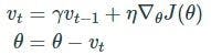
Momentum method

This method is used to reduce the fluctuations in the stochastic gradient descent algorithm by helping it move in the relevant direction. This is done by adding the update vector of the last step. The step factor is further multiplied by another constant that is usually set to a value close to 0.9.

Adagrad optimizer

Adagrad optimizer works well when dealing with sparse data as the algorithm performs small updates in the weights based on features that occur often. In Adagrad, different learning rates are used for every parameter update at every time step. The algorithm uses larger learning rates for infrequent features and small learning rates for frequent ones. The major advantage of using the Adagrad optimizer is that the learning rate need not be set manually. Note that when using the algorithm, the learning rate may shrink to almost 0. At this point, the model gains no new knowledge.

RMSprop

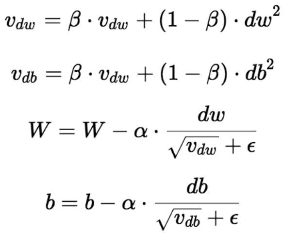
The RMSprop optimizer is similar to gradient descent with momentum and Adagrad optimizer, but it uses a different method for parameter update. In RMSprop, the oscillations in the vertical direction are restricted so that the algorithm can take larger steps in the horizontal direction. The algorithm uses a decaying moving average that allows it to focus on the most recent observed gradients. Moreover, the RMSprop uses an adaptive learning rate, which means that the learning rate is not a hyperparameter and it changes with time.

The image below shows the parameter update rule for RMSprop.

Adam optimizer

The Adam optimizer is the advanced version of the classical stochastic gradient descent algorithm that inherits the advantages of both Adagrad and the RMSprop optimization algorithms. It adapts the learning rates based on the average first momentum (mean) and the average second momentum (variance). Adam is a popular algorithm in the field of machine learning and deep learning and gives satisfactory results for most problems. It is used as the default algorithm in many cases and is recommended by professionals owing to its outstanding performance.

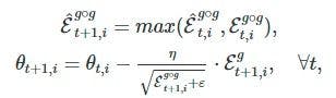
AMSGrad

Despite the advantages of the Adam optimizer, it does not converge to a simple optimization algorithm. To address the issue, the AMSGrad optimization algorithm was introduced. However, its performance is not superior to the Adam optimizer.

The image below shows the update rule for AMSGrad.

You can read more about AMSGrad here.

AdamW

This is a modified version of the Adam optimizer, which uses the concept of weight decay. It is widely used in machine learning to achieve better results. It implements L2 regularization in the Adam along with the modification below.

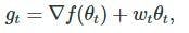
Here, wt represents the weight decay at time t.

Gradient descent is a great substitute for an exhaustive search algorithm. It is a brute force approach. It is used to update model parameters and reduce the loss function until it becomes 0 or the maximum iteration is reached. Different gradient descent algorithms can be used depending on the size of the dataset and the speed of training.

The motivation for each algorithm is to rectify the drawbacks of the previous benchmarks while improving its performance or, at the very least, keeping it the same. Even a basic algorithm can outperform an advanced one, depending on the requirements and the dataset.