Effects of Normalization Techniques on Logistic Regression in Data Science
•8 min read
- Languages, frameworks, tools, and trends

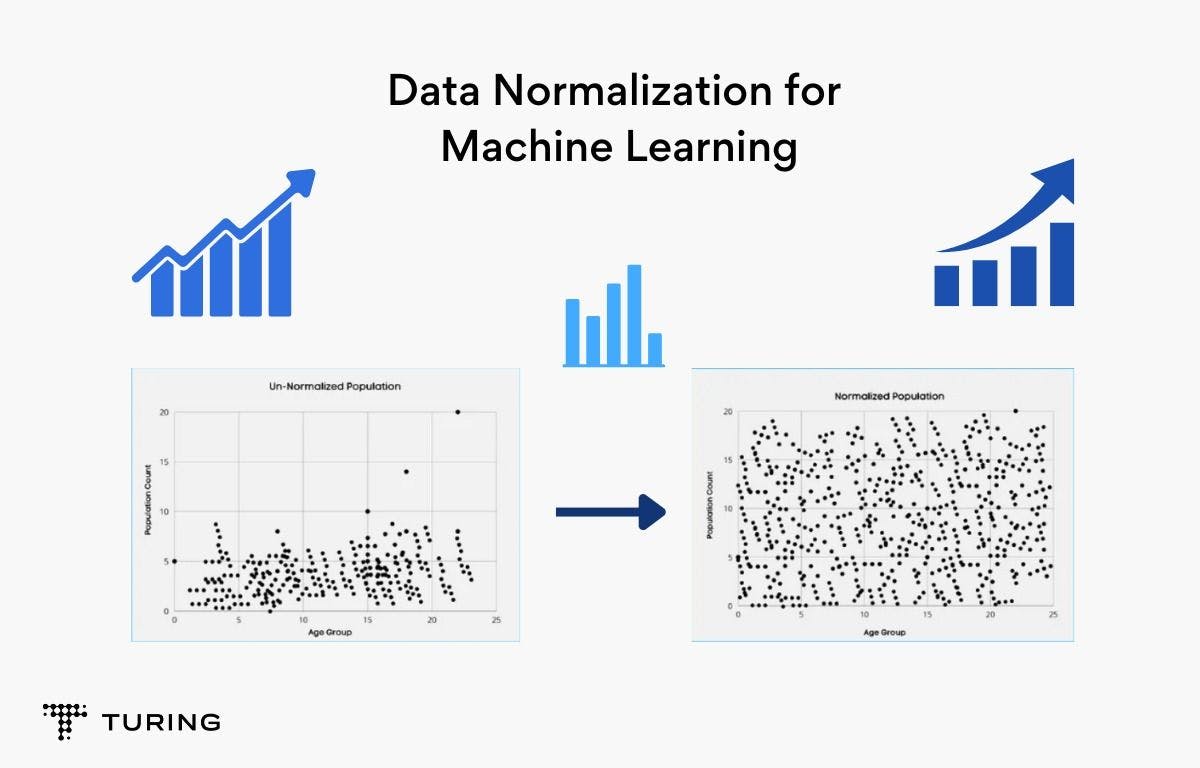
Advancements in data science have enabled the application of numerous mathematical concepts to data behavioral patterns. Different normalization techniques are applied to datasets to tackle problems in a variety of fields, and normalization itself is used as a pre-processing strategy in data mining methods.
This article will look at how normalization strategies affect the performance of a logistic (or logit) regression classifier in data science.
Logistic regression is an excellent algorithm for addressing classification problems. Since the goal of this article is to compare how different normalization techniques affect the performance of logistic regression models, the most used normalization methods - min-max, z-score are employed to transform the original data. The performance of the resulting models is evaluated using accuracies and model lifts as the primary metrics.
Methodology
A typical workflow entails creating a data model in Python and checking for its accuracy.
Dataset
A binary logistic regression model is developed in Python in the Jupyter Notebook to predict whether a patient has diabetes using binary logistic regression.
Before moving ahead, here’s a quick look at the basics of diabetes, which is a group of metabolic disorders characterized by hyperglycemia (high glucose levels). It’s divided into three types:
- Type 1 diabetes, which primarily affects children. Genetics and viruses may contribute to it.
- Type 2 diabetes, in which patients have insulin resistance or are unable to produce enough insulin. It’s the most common type of diabetes.
- Gestational diabetes, which affects pregnant women. Patients are unable to make enough insulin.
The dataset used was the Pima Indian Diabetes dataset from Machine Learning Repository (originally from the National Institute of Diabetes and Digestive and Kidney Disease), which contains eight medical diagnostic attributes and one target variable (i.e., Outcome) of 768 or 34.9% female patients with diabetes (268 patients).
For both groups, the insulin variance was relatively substantial. The values of diabetic and non-diabetic patients were compared using an independent t-test, which revealed that differences existed for all eight independent variables. As an example, data suggests that diabetics' average blood sugar concentration was on top of non-diabetics average blood sugar concentration. Mean=142.2 mg/dl (95 percent CI: 138.6, 145.7); t (766) = 15.67, p 0.001 at the 95% confidence level.

Overview of logistic regression
Unsupervised and supervised are the two types of machine learning techniques. For data dimensionality reduction, unsupervised learning techniques mostly involve grouping and regression, such as principal component analysis (PCA). The model output is predicted or categorized based on patterns in the input data using these unsupervised techniques, which do not require labeled data.
In contrast, supervised procedures require that the data be labeled and divided into training and testing datasets. Classification (training a model to determine which animal is in a shot) and regression are the two basic applications of supervised learning techniques (predicting the price of a house based on number of rooms, neighborhood, area, etc.). Supervised classification algorithms, on the other hand, cannot anticipate an animal that was not present during model training. The data is divided so that the model can be tested on data that it has never seen before, i.e., testing data). A confusion matrix can be constructed after a model has been fitted to evaluate the model in addition to other metrics.
Linear regression is a regularly used supervised regression technique in which an independent variable is used to estimate the dependent variable (i.e., hours of study to estimate grades). In multiple linear regression (MLS), this analogy can be extended to several independent variables being used to estimate a dependent variable (i.e., hours of study, extracurricular activity, number of days sick used to predict grades). In contrast to MLS, which produces a continuous value, e.g, property price or grades, logistic regression returns the likelihood of a binary result, for e.g., is an email spam or not?
Despite the name, logistic regression is a supervised classification algorithm. It’s used to estimate the probability that an occurrence belongs to a classification, e.g., spam folder of email, where a threshold probability of >50% predicts that the occurrence belongs to the positive class (denoted as 0, i.e. normal email) or predicts that the classification belongs to the negative class (denoted as -1, i.e. spam email, denoted as 1, i.e. spam). The logistic function is a sigmoid function whose output is restricted to a range of 0 to 1.
Many applications of logistic regression may be found in healthcare settings, such as predicting whether a disease is benign or cancerous based on nth factors. A database of patients with several variables is divided into two parts, with the training dataset used to train the model and the test dataset used to evaluate the model. These indicators can be used to determine if a new patient's cancer is benign or malignant. While binary logistic regression is the most common type of logistic regression, multinomial logistic regression can be used to predict membership in more than two categories, e.g., is a person married, single, or divorced.
There are several general assumptions that must be met to apply logistic regression.
- The true conditional probabilities are based on the independent variables' logistic functions.
- Independent variables are accurately measured.
- The observations are self-contained.
- Errors follow a binomial distribution.
- Independent variables aren't linearly related to one another.
- No irrelevant variables are included, and no critical factors are left out.
Even though many datasets contain nominal data, logistic regression cannot model these variables. Linear regression cannot either. To get around this, you can create a dummy variable. Perfect multicollinearity can be prevented by removing one of the data type's dummy variables. If the correlation coefficient of numerous independent variables is strong (>0.8), multicollinearity might affect the estimation of the dependent variables and the interpretation of the logistic regression model's independent coefficients.
Normalization techniques
The following section will cover the three different types of normalization algorithms used on the dataset. There are many different types of methods, but these three were chosen in order to see their effect on the logistic regression model. Min-max, z-score, and robust scaling are examples of these approaches.
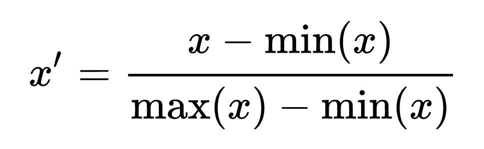
Min-max normalization
This method involves linearly transforming characteristics or outputs from one set of values to another set of values. The variables are usually modified to fall between 0 and 1 or -1 and 1. The linear transformation y = (x – min(x))/(max(x) – min(x)) is commonly used to rescale images. The minimum and maximum values in X are min and max, respectively, and X is the set of observed values of x. In other words, the range of X is max(x) – min(x). The benefit of this normalization method comes from the fact that all data associations are retained exactly.
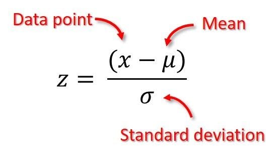
Z-score normalization
This is the most frequent normalizing approach. It converts all input values to a common measure with a standard deviation of one and an average of zero. Each attribute's mean and standard deviation are determined. The computed mean and standard deviation are used to normalize each value of an attribute X. y = (x – mean(X))/std is the transformation equation (X) where mean(X) is the attribute's mean, and std(X) is the attribute's standard deviation. The benefit of this strategy comes from the fact that it decreases the impact of outliers on the data.
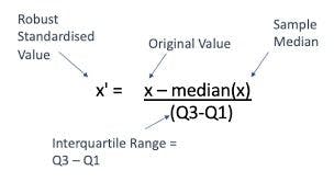
Robust scaling
The median is removed and the data is scaled according to the quantile range. The interquartile range (IQR) is the distance between the first and third quartiles (25th and 3rd quantiles) (75th quantile).
Structural representation of activities
The dataset is presented in four different formats and structures in the logistic regression model. The inputs to the model were the original dataset and the generated datasets after normalization using three alternative procedures as shown in the model above. As a result, four separate prediction models were created. Based on the model's prediction accuracies, the three outputs from the normalization procedures were compared to the output of the original dataset.
Results
The tests were carried out to determine how different normalization techniques affect the performance of the logistic regression model. The dataset was divided into two sets. The training set contains 80% of the original dataset (614 records) while the testing set contains the remaining 20% of the dataset (154 records). The diabetes dataset was normalized using the min-max, z-score, and robust scaling normalization methods. For each of the normalization techniques, the same percentages of training and testing sets were used.
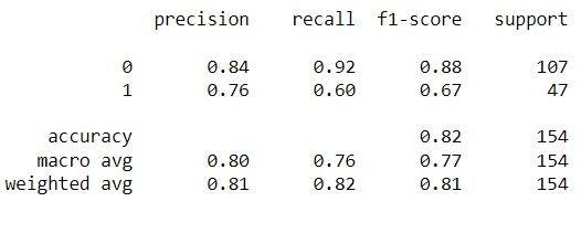
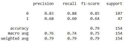
Classification matrix for baseline-model on quality
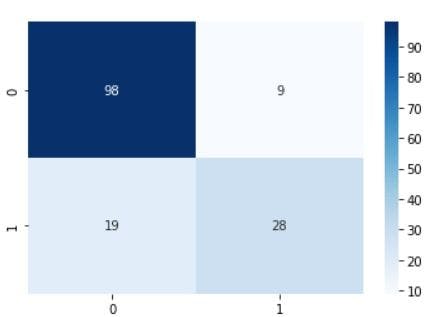
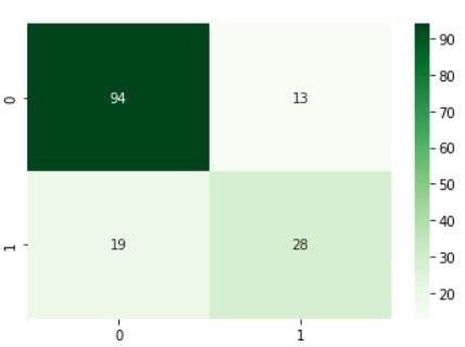
Confusion matrix for baseline-model on quality
The classification matrices for the four models are shown below, one for the original dataset and the other three for each normalizing procedure. These matrices, also known as confusion matrices, are used to summarize a classification algorithm or classifier's performance. The classification matrices' columns relate to actual values while the rows correspond to anticipated values.
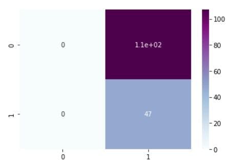
Classification matrix for min-max on quality
Confusion matrix for min-max on quality
Classification matrix for z-score-model on quality
Confusion matrix for z-score-model on quality
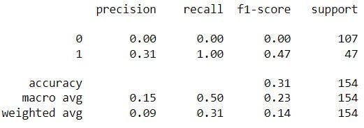
Classification matrix for robust scaling
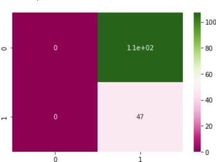
Confusion matrix for robust scaling
Accuracy
The percentage of the test dataset correctly provided is used to determine a model's accuracy. Accuracy is the number of correctly classified test samples. The total number of samples for testing the sum of all the diagonal values in a matrix equals the number of correctly identified test samples. The accuracies reported by the four models are listed below in the image.
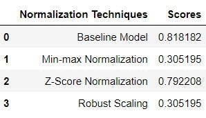
Models accuracy
Three alternative normalization procedures were used to evaluate the performance of the logistic regression model. Normalizing a dataset is intended to improve the predictive accuracy of a machine learning algorithm, yet logistic regression does not respond well to any of the three normalization strategies examined. Although the training datasets were of various sizes, the accuracies of both models based on the normalization procedures were comparable.