Deep Dive Into Chebyshev’s Inequality in Statistics

Chebyshev inequality in statistics is used to add confidence intervals (95%) for the mean of a normal distribution. It was first articulated by Russian mathematician Pafnuty Chebyshev in 1870. And it is known as one of the most useful theoretical theorem of probability theory. It is mainly used in mathematics, economics, and finance and helps in working with statistical data.

There are many statistical methods but Chebychev inequality is a statistical method that has been widely discussed in a lot of case studies and scenarios.

Chebyshev's rule calculator is a tool that can be used to calculate the influence of the data on the company by using this inequality method. It gives you an insight into how your product or service is performing based on the data you gather for your customers or clients. In this article, we specifically give an introduction to the Chebyshev inequality.

What is Chebyshev’s inequality?

Chebyshev's inequality is considered to be the fundamental result that lies at the basis of the theory of normal probability distributions — or even the whole of mathematical probability itself.

Chebyshev's inequality, also known as Bienayme-Chebyshev inequality in probability theory, can never be more than a given fraction of values that vary significantly from the average, regardless of the class of probability distribution.
For a large range of probability distributions, this is a probability theory that guarantees there are no more than a specified fraction of values within a specific range. Consequently, a small number of values will be close to the distribution mean.

In other words, no more than 1/k2 of a distribution's values can exceed its mean. The mean of distribution cannot be separated from its values by more than k standard deviations. Also, it indicates that values 1–(1/k2) of distribution must fall within k standard deviations of the distribution's mean, but not include it.

A big advantage of this theorem is that it is applicable to any probability distribution regardless of its normality, as long as the mean and variance are known. The theorem is as follows:

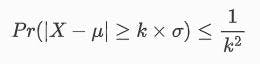
By using the formula, the probability of a value (X) being more than k standard deviations away from the mean, is less or equal to the probability of a value being more than k standard deviations away from the mean. It can have any value above zero, as it is a distance measured from the mean.

How to use Chebyshev's inequality formula?

Here are a few examples of the inequality for different values of k:

Taking k = 2 as an example, we have 1 - 1/k2 = 1 - 1/4 = 3/4 = 75. In other words, Chebyshev's inequality says that distribution is within two standard deviations of the mean for at least 75% of its values.

If k = 3, then 1 - 1/k2 = 1 - 1/9 = 8/9 = 89%. Furthermore, Chebyshev's inequality dictates that 85% of the value of distribution must fall within three standard deviations of it.

With k = 4, we have 1 - 1/k2 = 1 - 1/16 = 15/16 = 93.75%. Hence, Chebyshev's distributions require that at least 93.75% of the data values that must lie within two standard deviations of the mean.

How to solve problems using Chebyshev's inequality formula?

The more information we have about the distribution we're working with, the more likely we are to find data that's a certain number of standard deviations from the mean.

When the data is normally distributed, 99% of observations lie between +3 and - 3 standard deviations, while 97% lies between + 1 and - 1 standard deviations.

Thus, we can see that more than 75% of the data is centered around the mean. Taking this case into account, we can conclude that the percentage could be much higher than 75%. In this case, Chebyshev's inequality says that 75% of the data is two standard deviations off the mean.

This inequality provides us with a “worse case” scenario when we only know the means and standard deviations of our sample data (or probability distribution). When we are unaware of anything else about our data, Chebyshev's inequality can give us insight into how to spread it out.

Let's say that we sampled dogs at the local animal shelter and found that their weights ranged from 20 pounds to 3 pounds. In our sample, we know that 75% of the dogs had a weight two standard deviations above the mean because of Chebyshev's inequality. We get the square root of the standard deviation by multiplying it two times by six. By subtracting and adding the mean weight and the median weight, we find that 75% of the dogs weigh between 14 to 26 pounds.

How to calculate Chebyshev inequality with real-world data?

Take the example of an insurance company that provides different types of claims for its customers at different times and in varying amounts. Based on what you have received so far, you want to know how large the claims will likely be in the future. In order to cover the claims of the upcoming calendar year, for example, you need to set aside enough reserves.
So all claims are assumed to be independent and equally distributed. Therefore, each claim is considered to be based on a random drawing from a single unknown distribution.

It is clear from Chebyshev's inequality that you can be at least 90% sure that future claims will not be more than three standard deviations from their means. This is without knowing anything about the underlying distribution.

With the examples of the claims, you can estimate the mean and standard deviation pretty accurately. With Chebyshev's inequality, you can instantly get a 90% prediction interval for future claims without considering the underlying distribution (other than finite mean and variance, of course).

Next

If you give the claims a parametric structure, you can get much tighter prediction intervals for future claims. In the example above, if you assumed that the claims were drawn from the Gamma distribution, you could estimate the parameters of the Gamma distribution from your observations. With this method, you can compute a tighter 90% prediction interval than the one provided by Chebyshev's inequality.

Using this method, there's a small risk that the underlying distribution isn't Gamma at all. Your Gamma assumption may lead you to dangerously underestimate the sizes of future claims if the real distribution is log-normal, as in the case of Pareto distributions. As you know, the Gamma distribution has heavier tails than both these distributions do, so you would be incorrect in using it on the basis of your assumption. Despite Chebyshev's inequality giving you a wider prediction interval, it is much more reliable.

Applications of Chebyshev’s inequality

Combining calculus with the weak version of the law of large numbers helped to develop the formula. By law, a larger sample set should be closer to its real mean (i.e. the one expected in a population) as it increases in size. As an example, the probability average for rolling a six-sided die is 3.5.

The results of a sample size of five rolls may be drastically different. Upon rolling the die 20 times, you should begin to see an average approaching 3.5. If you keep rolling until it reaches 3.5, the average should continue to rise until it reaches that number. The result is pretty close to equal in either case.

You can also use it to find the difference between a collection of numbers' mean and median. A measure of standard deviation, respectively, is smaller or equal to the median-mean difference according to Chebyshev's inequality theorem, also known as Cantelli's theorem. This is helpful in determining whether the median you calculated is plausible.

As the sample size gets smaller, Chebyshev's inequality does not produce very accurate lower bounds. Random samples of large sizes are much more useful. Although these distributions are unrestricted, they are very weak since they tend to be very large. Therefore, it is rarely used in the real world.

Python implementation

In order to work with Chebyshev, we need to import a few libraries:

import numpy as np
import matplotlib.pyplot as plt
from scipy.stats import norm

A simple function can be written for Chebyshev's inequality:

def chebyshev_inequality(k):
    return 1 / k**2

Using this function, we can now calculate the probability for different values of k. Let's start by creating an array of 10 numbers with a distance between each value of 0.5. We'll also need an array of zero values of the same length to be able to hold the probability values we're about to calculate.

k = np.arange(10,20,0.7)
p_cheb = np.zeros(len(k))

print('Chebyshev_Inequality for different k values:\n') 

for i in range(len(k)):
    p_cheb[i] = chebyshev_inequality(k[i])
    print(f'Pr( |𝜇−𝜎| >= {k[i]}𝜎 ) <= {p_cheb[i]}' )

Output

Once we are done with writing code, its time to execute it. When you execute it as given, you will get output like below.

Chebyshev_Inequality for different k values:

Pr( |𝜇−𝜎| >= 10.0𝜎 ) <= 0.01
Pr( |𝜇−𝜎| >= 10.7𝜎 ) <= 0.008734387282732119
Pr( |𝜇−𝜎| >= 11.399999999999999𝜎 ) <= 0.007694675284702987
Pr( |𝜇−𝜎| >= 12.099999999999998𝜎 ) <= 0.006830134553650709
Pr( |𝜇−𝜎| >= 12.799999999999997𝜎 ) <= 0.0061035156250000035
Pr( |𝜇−𝜎| >= 13.499999999999996𝜎 ) <= 0.005486968449931415
Pr( |𝜇−𝜎| >= 14.199999999999996𝜎 ) <= 0.004959333465582229
Pr( |𝜇−𝜎| >= 14.899999999999995𝜎 ) <= 0.004504301608035677
Pr( |𝜇−𝜎| >= 15.599999999999994𝜎 ) <= 0.004109138724523343
Pr( |𝜇−𝜎| >= 16.299999999999994𝜎 ) <= 0.003763784862057288
Pr( |𝜇−𝜎| >= 16.999999999999993𝜎 ) <= 0.00346020761245675
Pr( |𝜇−𝜎| >= 17.699999999999992𝜎 ) <= 0.0031919307989402815
Pr( |𝜇−𝜎| >= 18.39999999999999𝜎 ) <= 0.002953686200378075
Pr( |𝜇−𝜎| >= 19.09999999999999𝜎 ) <= 0.002741152928921907
Pr( |𝜇−𝜎| >= 19.79999999999999𝜎 ) <= 0.0025507601265177047

Implementation of Chebyshev inequality theory for non-coders

The formula can only be used to calculate results for standard deviations greater than 1; it cannot be used to calculate results for standard deviations as small as 0.1 or 0.9. Although, it is technically possible to use this formula and get some results, but it would not be valid.

Example problem:

The mean and standard deviation of a left-skewed distribution are 4.99 and 3.13 respectively. According to the following formula, at least two standard deviations should separate observation from the mean:

Step 1: Square the number of standard deviations:

22 = 4.

Step 2: Divide 1 by the answer you got in step 1:

1 / 4 = 0.25.

Step 3: Subtract step 2 from 1:

1 – 0.25 = 0.75.

The mean standard deviation of nearly half the observations is between -2 and +2.

That’s:

mean: – 2 standard deviations

4.99 – 3.13(2) = -1.27

mean: + 2 standard deviations

4.99 + 3.13(2) = 11.25

Or between -1.27 and 11.25

That’s it!

Calculate Chebyshev's Formula in Excel

Microsoft Excel and Google Spread sheets come with many built-in formulas and functions that make it easy to perform statistical calculations. It however lacks the Chebyshev's theorem formula. Adding the formula to Excel is the only way to calculate the theorem. If you plan to use it only once or twice, you can type the formula into a cell. And in case you are planning to use the formula more than once, you can add a custom function (=CHEBYSHEV) to Microsoft Excel.

Step 1: Type the following formula into cell A1: =1-(1/b1^2).

Step 2: Type the number of standard deviations you want to evaluate in cell B1.

Step 3: When you press the enter key, Excel returns the percentage of results you can expect to find within that number of standard deviations in cell B1.

There are several interesting facts about data sets that can be proven through Chebyshev's inequality. In probability, Chebyshev's inequality is a fundamental rule. You can easily find out whether a variable follows a certain distribution. The method also enables you to determine how a variable's value changes over time as a result of changing the mean, standard deviation, and variance.

This method can also be applied in many different scenarios. It is similar to analyzing statistics to come up with an answer rather than just getting a vague idea from a graph. The Chebyshev inequality can be used to understand what the long-term average means, a probability calculation, the speed of something occurring, and how error can affect statistics.

The rule lets us determine whether there will be a steady decline, an increase, or a change in speed before the decrease continues. This rule can give you the answer within one degree of error (if you don't worry about it increasing further).

FAQ

1. What is the difference between empirical rule and Chebyshev's theorem?

Chebyshev's theorem does not make any assumptions about the distribution. It is applicable to all types of data distributions, while the Empirical Theorem assumes that the data is normally distributed.

A lower bound for the proportion of data inside an interval symmetric about the mean can be found using Chebyshev's inequality theorem, whereas the approximate amount of data within an interval can be found using the Empirical theorem.

With the Empirical Rule, bell-shaped relative frequency histograms can be approximated for data sets. A standard deviation of one, two, or three is calculated based on the proportion of measurements that fall within these ranges. Whereas, Chebyshev's Theorem applies to any and all data sets. It indicates a minimum percentage of measurements that should lie within one, two, or more standard deviations from the mean.

2. Does Chebyshev's inequality apply to all distributions?

Chebyshev's inequality and the 68-95-99.7 rule have much in common; the latter rule applies to normal distributions only. Chebyshev's inequality applies to any distribution as long as the variance and mean are defined.

3. How do you calculate the Chebyshev interval?

Let’s consider the following example to understand this. You have a distribution with following characteristics:

• Mean = 100
• Standard deviation = 10

With the above data, you want to find a range of data that lies between + 2 and - 2 standard deviations. Thus, 2 standard deviations mean 2 * 10 = 20.

Further, according to Chebyshev's theorem, 75% data would fall between 100 + 20 and 100 - 20. Thus, the requisite interval would be 80 - 120.