Understanding Methods of ANNs - Particle Swarm Optimization, Backpropagation, and Neural Networks

The advancement of machine learning has brought the artificial neural network (ANN) into limelight. The latter takes inspiration from the human brain and has been widely used for solving real-world problems. This article will cover the methods involved in ANNs like particle swarm optimization, backpropagation, and neural networks.

Artificial neural networks

Artificial neural networks (ANNs) or neural networks are the most researched area in the field of artificial intelligence. The neural networks has three sets of operations:

1. The first set is the pattern of connection between the different neurons in the architecture.

2. The second set is the method that is used for determining the weights of the connections.

3. Finally, the last set is the activation function which is important to limit the output amplitude of the neurons.

Backpropagation is a popular method of artificial neural networks. This technique involves a network of nodes that are arranged in layers. The first layer is called the input layer, and the last layer is called the output layer. And the layers in between these two are called hidden layers.

Steps of backpropagation algorithm

The backpropagation algorithm involves the following steps:

1. The input layer gets presented to an input vector.

2. The output layer gets presented to the set of the desired output.

3. Comparison is made between the desired output and the actual output, that is how the error is calculated.

4. The comparison determines weight changes according to learning rules.

Drawbacks of backpropagation algorithm

The major disadvantage of using this technique is that it takes a lot of time to train the models. This is mainly because the neurons performs backward to achieve the ideal solution. This has limited its usage and persuaded researchers to come up with a better and replacing technique known as particle swarm optimization.

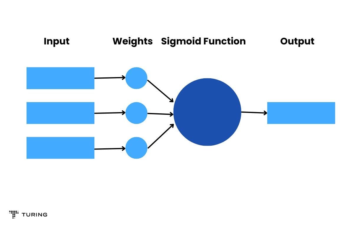
The architecture of the neural network is shown in Fig. 1. Each node comprises an activation function called Sigmoid function (or other functions like ReLU). The input node is responsible for sending the signal that passes through a weighted connection and the output is produced according to the internal activation function.

Backpropagation Algorithm (BP)

Fig. 2 shows the Multilayer Perceptron (MLP) architecture.

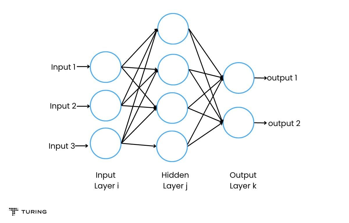
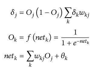
The input is processed from input layer i and processed to hidden layer j. This can be mathematically represented by the following equation:

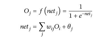
Eq. (1)

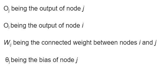
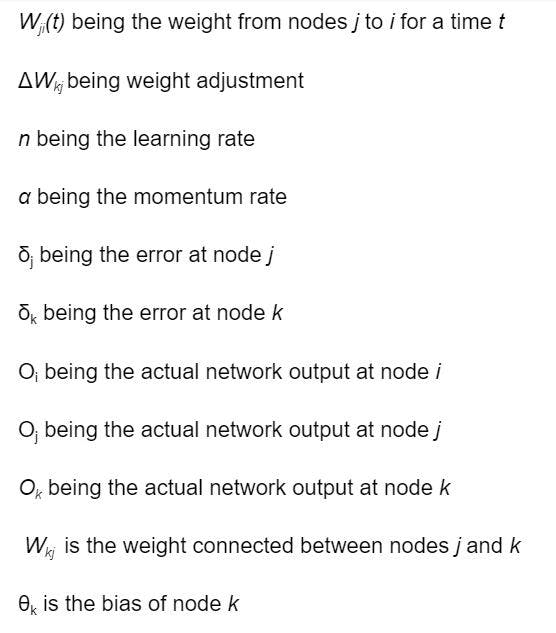
Where:

Similarly, the transition from hidden layer j moves to the final layer i.e. the output layer using the Eq. (1).

Now, once the output is produced, an error can be calculated using Eq. (2). It compares the actual output with the desired output. Thus, the error gets propagated in the backward direction starting from the output layer to the hidden layer and then to the input layer. Thus, the weights are modified and error is minimized.

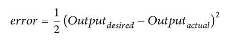
Eq. (2)

Once the error is calculated, the backpropagation algorithm is applied from output node k to hidden node j as shown in Eq. (3):

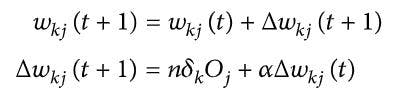
Eq. (3)

Where,

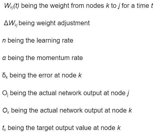
The backpropagation algorithm from the hidden layer j to the input layer i is calculated as follows:

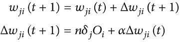
Eq. (4)

Where,

Where,

This process is continued till convergence is achieved, thereby making it a longer process. This is the reason, it is a less preferred technique compared to particle swarm optimization.

Swarm intelligence

This technique was developed by Konstantinos and Michael in 2009. It aims to find a global solution with all the neurons that work as a team to find the best resting place. This technique has been inspired by the flock of birds where each bird contributes to reach the destination.

Swarm intelligence comprises two major algorithms namely ant colony optimization (ACO) and particle swarm optimization (PSO). In the ant colony optimization (ACO) technique, the optimal solution is found using graphs that are inspired by ants finding ways from their colony to food. In particle swarm optimization (PSO), all particles (i.e. neurons) work as a team to find better results.

Particle swarm optimization

In PSO, the basic workflow is illustrated in the Fig. (3) given below -

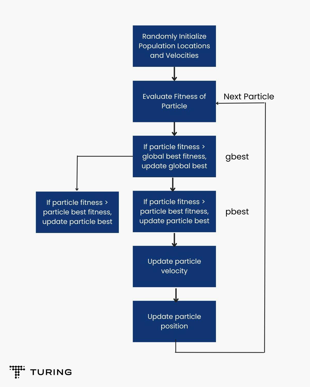
In this technique, all swarms (neurons) move together to find the global solution where the position of these swarms are updated by a vector called velocity vector.

According to many researchers, few modifications can be made in the following categories:

1. The extension of field searching space,
2. Adjustment of the parameters, and
3. Hybridization with another technique.

In PSO, each particle is assigned to a random position. The velocity of the physical position of particles are not important. All particles work as a team to find an effective solutions, they keep a record of each position they have taken. From all the obtained values, personal best value (pbest) and global best value (gbest) is obtained. During each iteration, particles move towards vectors pbest and gbest, which are weighted randomly altering the upcoming next positions of the particle.

There are two sets of equations involved in this technique is called equation of movements (Eg. (5)) and equation of velocity update (Eq.(6)).

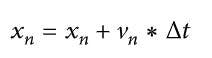
Eq. (5)

Eq. (6)

This equation of movements specifies the movement of particles using a specific vector velocity. The velocity update equation, on the other hand, provides velocity vector modification given by the two vectors (pbest and gbest).In Eq.(5), Δt species the time in which the swarm will be moving, and it is usually set to 1.0. This results in the new position of the swarm. In Eq.(6), subtraction of the dimensional element from the best vector, pbest, and gbest, is done which is further multiplied with a random variable between 0 to 1, and also with an acceleration constant of C1 and C2.

Thus, the sum gets added to velocity. The random variable helps to achieve randomness in the movement of particles throughout the solution space. Acceleration constants provide control to the equation that defines movement of particles towards pbest or gbest. To minimize the learning error of the results, the mean squared error is calculated. With the particle swarm technique, it is easier to approach the global solution in a shorter time and hence, it is a more preferred method than backpropagation.