Regularization Techniques in Deep Learning: Ultimate Guidebook

When a machine learning model is provided with training samples along with corresponding labels, the model will start to recognize patterns in the data and update the model parameters accordingly. The process is known as training. These parameters or weights are then used to predict the labels or outputs on another set of unseen samples that the model has not been trained on, i.e., the testing dataset. This process is called inference.

Correct fit vs. overfit models

If the model is able to perform well on the testing dataset, the model can be said to have generalized well, i.e., correctly understood the patterns provided in the training dataset. This type of model is called a correct fit model. However, if the model performs really well on the training data and doesn’t perform well on the testing data, it can be concluded that the model has memorized the patterns of training data but is not able to generalize well on unseen data. This model is called an overfit model.

To summarize, overfitting is a phenomenon where the machine learning model learns patterns and performs well on data that it has been trained on and does not perform well on unseen data.

Image source

Image source

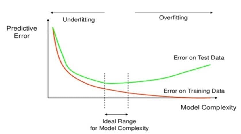
The graph shows that as the model is trained for a longer duration, the training error lessens. However, the testing error starts increasing after a specific point. This indicates that the model has started to overfit.

Methods used to handle overfitting

Overfitting is caused when the training accuracy/metric is relatively higher than validation accuracy/metric. It can be handled through the following techniques:

1. Training on more training data to better identify the patterns.
2. Data augmentation for better model generalization.
3. Early stopping, i.e., stop the model training when the validation metrics start decreasing or loss starts increasing.
4. Regularization techniques.

In these techniques, data augmentation and more training data don’t change the model architecture but try to improve the performance by altering the input data. Early stopping is used to stop the model training at an appropriate time - before the model overfits, rather than addressing the issue of overfitting directly. However, regularization is a more robust technique that can be used to avoid overfitting.

Types of regularization techniques

Regularization is a technique used to address overfitting by directly changing the architecture of the model by modifying the model’s training process. The following are the commonly used regularization techniques:

1. L2 regularization
2. L1 regularization
3. Dropout regularization

Here’s a look at each in detail.

L2 regularization

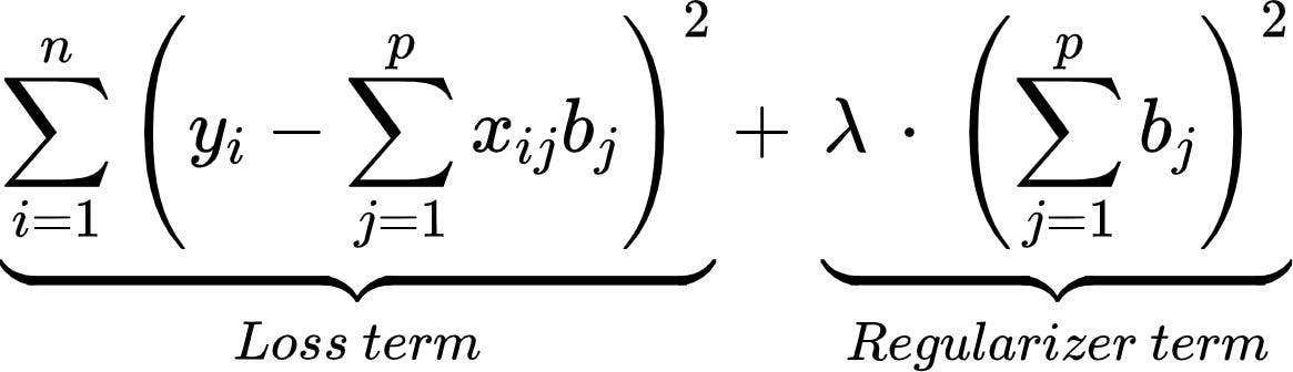
According to regression analysis, L2 regularization is also called ridge regression. In this type of regularization, the squared magnitude of the coefficients or weights multiplied with a regularizer term is added to the loss or cost function. L2 regression can be represented with the following mathematical equation.

Loss:

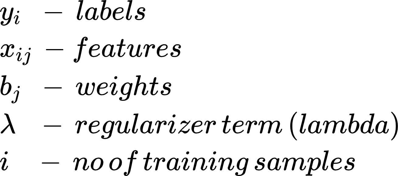
In the above equation,

You can see that a fraction of the sum of squared values of weights is added to the loss function. Thus, when gradient descent is applied on loss, the weight update seems to be consistent by giving almost equal emphasis on all features. You can observe the following:

• Lambda is the hyperparameter that is tuned to prevent overfitting i.e. penalize the insignificant weights by forcing them to be small but not zero.
• L2 regularization works best when all the weights are roughly of the same size, i.e., input features are of the same range.
• This technique also helps the model to learn more complex patterns from data without overfitting easily.

L1 regularization

L1 regularization is also referred to as lasso regression. In this type of regularization, the absolute value of the magnitude of coefficients or weights multiplied with a regularizer term is added to the loss or cost function. It can be represented with the following equation.

Loss:

In the above equation,

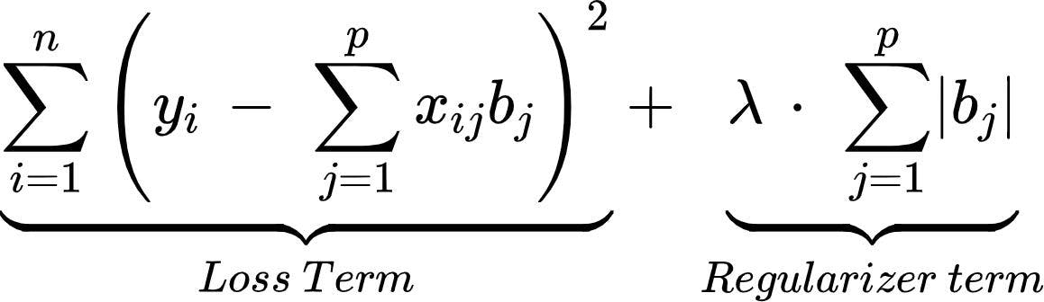
A fraction of the sum of absolute values of weights to the loss function is added in the L1 regularization. In this way, you will be able to eliminate some coefficients with lesser values by pushing those values towards 0. You can observe the following by using L1 regularization:

• Since the L1 regularization adds an absolute value as a penalty to the cost function, the feature selection will be done by retaining only some important features and eliminating the lower or unimportant features.
• This technique is also robust to outliers, i.e., the model will be able to easily learn about outliers in the dataset.
• This technique will not be able to learn complex patterns from the input data.

Dropout regularization

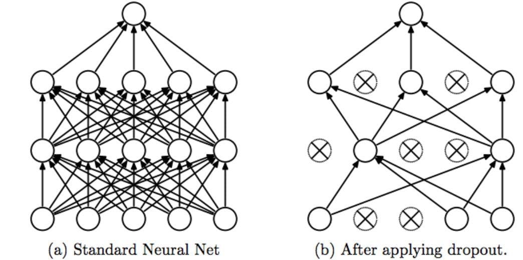
Dropout regularization is the technique in which some of the neurons are randomly disabled during the training such that the model can extract more useful robust features from the model. This prevents overfitting. You can see the dropout regularization in the following diagram:

• In figure (a), the neural network is fully connected. If all the neurons are trained with the entire training dataset, some neurons might memorize the patterns occurring in training data. This leads to overfitting since the model is not generalizing well.
• In figure (b), the neural network is sparsely connected, i.e., only some neurons are active during the model training. This forces the neurons to extract robust features/patterns from training data to prevent overfitting.

Image source

Image source

The following are the characteristics of dropout regularization:

• Dropout randomly disables some percent of neurons in each layer. So for every epoch, different neurons will be dropped leading to effective learning.
• Dropout is applied by specifying the ‘p’ values, which is the fraction of neurons to be dropped.
• Dropout reduces the dependencies of neurons on other neurons, resulting in more robust model behavior.
• Dropout is applied only during the model training phase and is not applied during the inference phase.
• When the model receives complete data during the inference time, you need to scale the layer outputs ‘x’ by ‘p’ such that only some parts of data will be sent to the next layer. This is because the layers have seen less amount of data as specified by dropout.

These are some of the most popular regularization techniques that are used to reduce overfitting during model training. They can be applied according to the use case or dataset being considered for more accurate model performance on the testing data.