Designing of Different Kernels in Machine Learning and Deep Learning

Before learning how to design kernels, it’s important to know the basic concepts related to kernels. A kernel can be defined as a function or a method that allows the application of linear methods to real-world problems that are nonlinear in nature. It does this by transforming data into higher dimensional spaces without explicitly computing in the high-dimensional feature space.

There are well-developed algorithms for machine learning and statistics for linear problems. Real-world data usually requires non-linear methods for making successful predictions of properties of interest. Thus, kernels are used in such types of datasets.

The kernel is said to be a dot product in a higher dimensional space where estimation methods are linear methods.

The history of kernels

The concept of kernels was first introduced into pattern recognition by Aizerman et al. (1964). It was in context to potential functions because of its analogy with electrostatics. It was subsequently neglected for many years until it was reintroduced into machine learning in the context of large margin classifiers by Boser et al. (1992). This led to the rise of a new technique called support vector machines.

This article will demonstrate how different kernels can be designed from the beginning.

Why are kernels necessary?

A common question that comes to mind when discussing kernels is why they’re needed in the first place. Here’s a look using an example.

There are two vectors, X (represented by green dots) and X' (represented by blue dots) in Fig.1.

Fig. 1

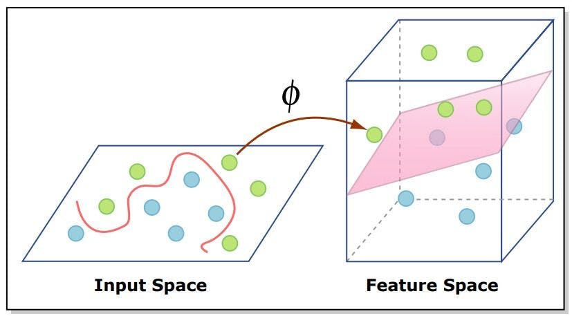
Fig. 1

It’s evident that the vectors X and X' are randomly distributed in a two-dimensional space and are difficult to separate using linear classifiers. However, the classification of the above dataset would require fitting of polynomial function - which requires expensive calculation - thus, complicating the problem of classification.

Keeping these challenges in mind, the problem can be easily resolved if the two vectors X and X' are transformed from a two-dimensional space to a three-dimensional one that is easily separable using a linear classifier. This is depicted in Fig.1 where the data is transformed from a two-dimensional space to a three-dimensional space with the help of a function, Φ. It can be represented as follows:

X → Φ(X)

X’ → Φ(X’)

Construction of kernels

Let’s define a simple kernel function as follows:

K(X, X’) = (X. X’)^2…………………………………………...................................................................................……………(Eq. 1)

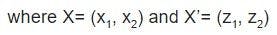
In Eq.1, K(X,X’) is a kernel function equivalent to the square of the dot product of two vectors, X and X’. It is further computed as follows:

Solving R.H.S. of Eq.1,

Thus, K(X, X’) = Φ(X) . Φ(X’)...................................................................(Eq.2)

From Eq.2, the kernel function can be defined as the dot product of two three-dimensional vectors. It shows how easily one can transform a dataset from a two-dimensional to a higher dimensional space without visualizing it.

The inner product of mapping functions rather than the data itself is commonly known as kernel trick or kernel substitution.

One of the most important and powerful techniques for creating new kernels is to use simpler kernels as fundamental building blocks. This can be implemented using techniques shown in Fig. 2.

Fig. 2

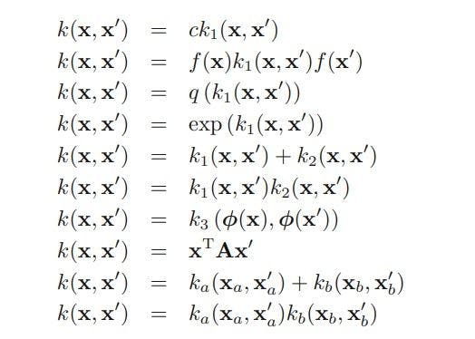
Fig. 2

From Eq. 2, it can be seen that the simple polynomial kernel has terms of degree two. Considering the more generalized form of kernels, it can be mathematically represented as:
(X’. X + c)^2
where c>0, then Φ(X) will have terms that are constant as well as terms of degree two. For instance, if a more generalized form of kernel is taken, which is (X’. X + c)^M, it will have all monomials of degree M.

Apart from the simple kernel shown above, another commonly used kernel is as below:

.........(Eq. 3)

This type is commonly known as a Gaussian kernel. Upon expanding the square of ||X-X’||, the result is:

.........(Eq. 4)

Thus, on substituting the Eq. 4 in Eq. 3, the result is:

...............(Eq. 5)

A significant contribution has been made in the kernel viewpoint that apart from vectors of real numbers as an input, kernel functions are defined over range objects such as graphs, sets, strings and text documents. For instance, consider that there is a fixed set and all possible subsets of this set are present there in a non-vectorial space. If A1 and A2 are such subsets, then:

where A1 ∩ A2 denotes the intersection of sets A1 and A2. and |A| denotes the number of subsets in A.

Generative models and discriminative settings

There’s another way to construct a powerful kernel: by applying generative models in a discriminative setting. Generative models are those that can generate their own data instances and can deal naturally with the missing data, while discriminative models discriminate between different kinds of instances of data. For example, generative models can generate instances similar to a particular kind of object like a car whereas discriminative models can easily distinguish between a car and an airplane.

In a more formal language, a generative model can be defined, for a given set of data X and a set of labels Y, as a joint probability of P(X,Y) or just P(X). On the other hand, a discriminative model can be defined as a conditional probability P(Y | X). It would be interesting to combine both models by first defining a kernel using a generative model and then using it in a discriminative approach.

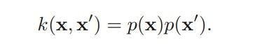
A kernel using a generative model can be defined as follows:

The above class of kernels can be further extended by considering sums over products of different probability distributions and positive weighting coefficients p(i), which can be represented as follows:

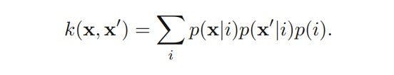
In the above kernel, two inputs, X and X’, will give large values if they have a significant probability under a range of different components.

As described above, it can be concluded that kernels play a major role in designing models as they help operate them in a higher dimensional space without visualizing them.